Chaotic Data: Correlation Dimension

Requires a Wolfram Notebook System
Interact on desktop, mobile and cloud with the free Wolfram Player or other Wolfram Language products.
This Demonstration shows how to infer the so-called correlation dimension for four chaotic datasets (each of length 4000). The data is derived from the logistic, Hénon and Lorenz models and NMR laser data. The log-log figure on the left contains the so-called correlation sums for some embedding dimensions  (as functions of a distance
  ). They are calculated at discrete points, which are connected with lines. (The correlation sums were calculated outside of this Demonstration because the computation takes too long; for these computations, see "Analysis of Chaotic Data with Mathematica" in the Related Links.)
Contributed by: Heikki Ruskeepää (April 2017)
Open content licensed under CC BY-NC-SA
Snapshots


Details
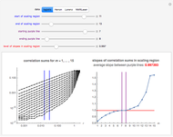
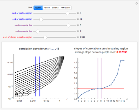
Snapshot 1: Logistic data. The figure on the left shows a scaling region between the eleventh and thirteenth values of . The slopes of the linear fits for the points between the two blue lines are given in the figure on the right. There, we can see that the slope approaches a value of approximately 0.997 when the embedding dimension increases from 1 to 7 and remains approximately the same for  . Thus, the value 0.997 seems to be a saturating value. This is our estimate of the correlation dimension. The correlation dimension of the logistic model is
  [1, p. 417]; our estimate is close to the actual value. Sprott [1] also mentions that the correlation dimension converges slowly for the logistic model.
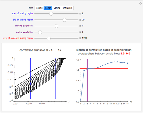
Snapshot 2: Hénon data. A scaling region seems to be between the eighth and twentieth values of . The slopes of linear fits of these points are approximately constant for  . The average of these slopes, 1.218, is the estimate of the correlation dimension. The correlation dimension of the Hénon model is
  [1, p. 422]; that is, the correlation exponent is in the interval
  . Our estimate of 1.218 is inside this interval.
Snapshot 3: Lorenz data. A scaling region seems to be between the eighth and nineteenth values of . The slopes of linear fits of these points are approximately constant for  . The average of these slopes, 2.021, is the estimate of the correlation dimension. The correlation dimension of the original continuous Lorenz system is
  [1, p. 431]; that is, the correlation dimension is in the interval
  . Our estimate 2.021 of the correlation dimension based on the sampled Lorenz system is inside this interval.
Snapshot 4: NMR laser data. A scaling region seems to be between the sixth and thirteenth values of . The slopes of linear fits of these points are approximately constant for  . The average of these slopes, 1.441, is the estimate of the correlation dimension.
These four settings are set as bookmarks in the "Bookmarks/Autorun" menu.
Correlation Dimension
The correlation dimension is a generalization of the usual integer-valued dimension. It gives a fractional dimension for the strange attractor. For nonchaotic data, the correlation dimension is the same as the usual dimension.
The correlation dimension can be estimated with the method of correlation exponent, as follows. Prepare the -dimensional delay coordinates  . Let
. Let  be the number of the delayed points
  . Define
  the number of pairs
  ,
,  , whose distance is smaller than . Then define
  to be the corresponding relative frequency:
 .
.
Thus, , also called the correlation sum, represents the probability that a randomly chosen pair of points in the reconstructed phase space will be less than a distance apart. The correlation exponent is the slope of  versus
  . To estimate the correlation dimension, we estimate the correlation exponent for increasing . If the correlation exponent saturates with increasing , the system is considered to be chaotic, and the saturation value is called the correlation dimension of the attractor.
Program for Correlation Sums
The correlation sums were calculated outside of this Demonstration. They can be calculated with the following program:
correlationSum[data_, τ_, mMax_, minΔt_Integer?(# >= 1 &), minExp_, maxExp_, nExp_] := Table[Module[{emb, nn, ed, bin, di}, emb = ParallelTable[Take[data, {i, i + τ (m - 1), τ}], {i, Length[data] - τ (m - 1)}]; nn = Length[emb]; ed = Flatten[ParallelTable[di = emb[[i]]; EuclideanDistance[di, #] & /@ Take[emb, {i + minΔt, nn}], {i, nn - minΔt}]]; bin = N@Binomial[nn - minΔt + 1, 2]; {10.^#, Total[UnitStep[(10.^#) - ed]]/bin} & /@ Range[minExp, maxExp, (maxExp - minExp)/(nExp - 1)]], {m, mMax}]
Here are the appropriate commands to calculate the correlation sums for the four datasets:
logistic = correlationSum[data, 1, 15, 20, -3.3, 0.3, 25]
Henon = correlationSum[data, 1, 15, 30, -3, 0.8, 25]
Lorenz = correlationSum[data, 16, 25, 600, 0, 1.8, 25]
NMRLaser= correlationSum[data, 1, 10, 200, 2, 4.2, 25]
A typical computing time is approximately two minutes.
We used the same four datasets (each containing 4000 values) as in "Chaotic Data: Delay Time and Embedding Dimension"; see Related Links. For each dataset, we also used here the value of the delay time  that we obtained in that Demonstration (these delay times are 1, 1, 16, and 1 for the four datasets, respectively).
Related Works
For details and other references, see Analysis of Chaotic Data with Mathematica. In that work, we estimate the delay time, embedding dimension, maximal Lyapunov exponent and also consider prediction.
In the Demonstration Chaotic Data: Delay Time and Embedding Dimension, we estimate the delay time and embedding dimension for the same four datasets. In the Demonstration Chaotic Data: Maximal Lyapunov Exponent, we estimate the maximal Lyapunov exponent.
Reference
[1] J. C. Sprott, Chaos and Time-Series Analysis, Oxford, UK: Oxford University Press, 2003.
Permanent Citation
 Chaotic Data: Delay Time and Embedding Dimension
Heikki Ruskeepää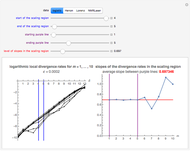 Chaotic Data: Maximal Lyapunov Exponent
Heikki Ruskeepää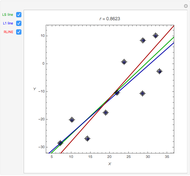 Correlation and Regression Explorer
Ian McLeod (The University of Western Ontario) Data Smoothing
Jon McLoone Grouping Country Data
Seth J. Chandler Edgeworth Expansion for Near-Normal Data
Housam Binous, Mamdouh Al-Harthi, and Brian G. Higgins Data Sampling and Interpolation
Brian Van Vertloo Rasterization of a Data Plot
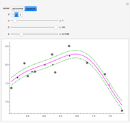
Paul van der Schaaf Local Regression for Country Data
Heikki Ruskeepää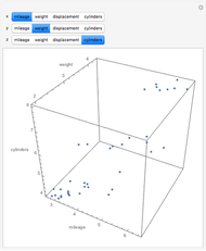 Visualizing Higher-Dimensional Data with 3D Scatterplots
Ian McLeod
-
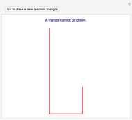
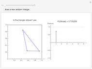 Obtuse Random Triangles from Three Points in a Rectangle
Heikki Ruskeepää -
Chaotic Data: Maximal Lyapunov Exponent
Heikki Ruskeepää -
 Chaotic Data: Correlation Dimension
Heikki Ruskeepää -
Chaotic Data: Delay Time and Embedding Dimension
Heikki Ruskeepää -
 Method of Support Vector Regression
Heikki Ruskeepää -
Local Regression for Country Data
Heikki Ruskeepää -
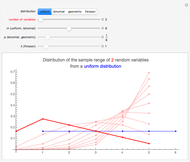
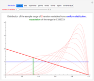 Distribution of the Sample Range of Continuous Random Variables
Heikki Ruskeepää -
 Distribution of the Sample Range of Discrete Random Variables
Heikki Ruskeepää -
 Distributions of Discrete Order Statistics
Heikki Ruskeepää -
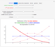
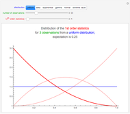 Distributions of Continuous Order Statistics
Heikki Ruskeepää -
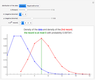
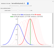
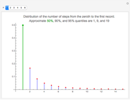 Waiting for the Next Record
Heikki Ruskeepää -
 Distribution of Discrete Records
Heikki Ruskeepää -
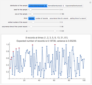 Records in Sequences of Random Variables
Heikki Ruskeepää -
 Distribution of Records
Heikki Ruskeepää -
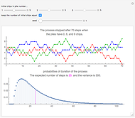 The Three-Tower Problem
Heikki Ruskeepää -
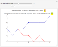 Walking Randomly Until No Shoes Are Available
Heikki Ruskeepää -
 A Reluctant Random Walk
Heikki Ruskeepää -
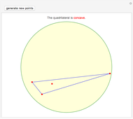 Concave Random Quadrilaterals from Four Points in a Disk
Heikki Ruskeepää -
 Obtuse Random Triangles from Three Parts of the Unit Interval
Heikki Ruskeepää -
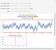
 Spin Game
Heikki Ruskeepää