Charged Particle Subjected to Lorentz Force: Analytical Solution


Requires a Wolfram Notebook System
Interact on desktop, mobile and cloud with the free Wolfram Player or other Wolfram Language products.
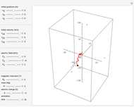
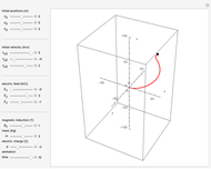
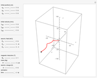
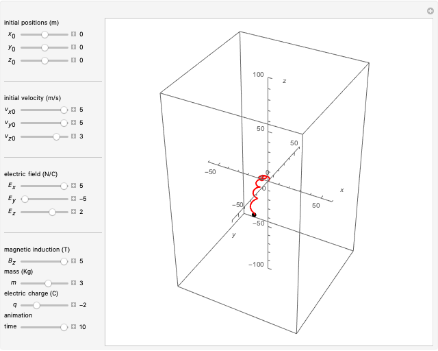
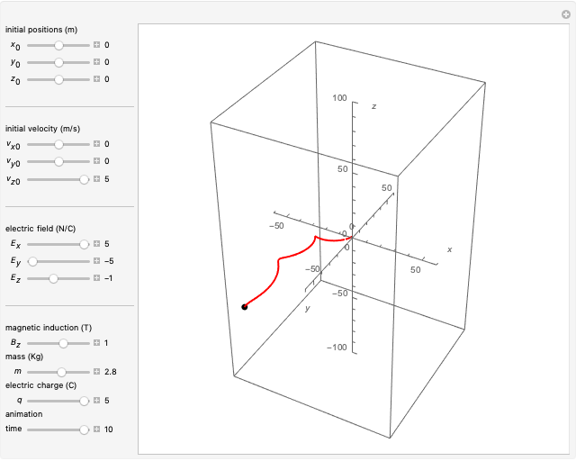
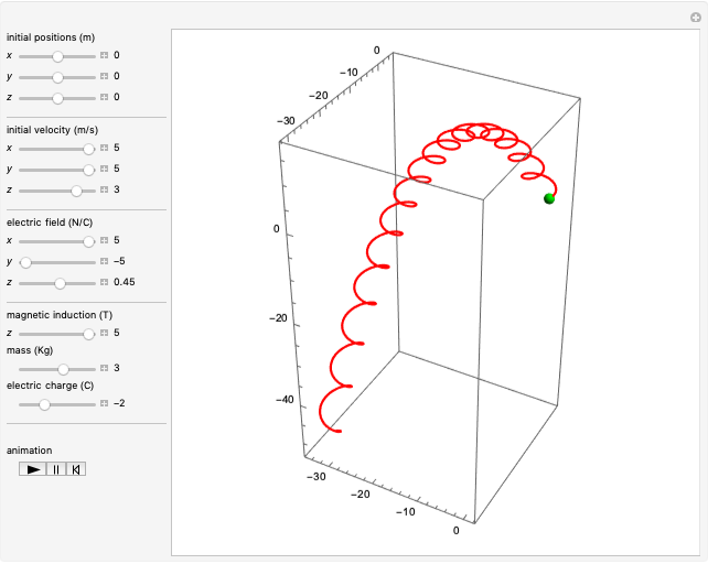
When subjected to electric and magnetic fields, the motion of a Newtonian particle depends on the Lorentz force. This Demonstration describes the effect of a homogeneous magnetic field in the  direction combined with a homogeneous electric field in an arbitrary direction on the trajectory of a charged particle, given its charge, mass, initial position and initial velocity. This is done analytically, with the solution described in the Details.
Contributed by: Deyvid W. M. Pastana, Vinicius B. Neves, Manuel E. Rodrigues and Luciano J. B. Quaresma (April 2020)
Open content licensed under CC BY-NC-SA
Snapshots

Details
Considering a particle of charge  and mass
  , subjected to an electric field
 ,
,
and a magnetic field
 ,
,
the resulting force  is given by the Lorentz force:
 .
.
In Cartesian coordinates the position vector is
 ,
,
then the velocity is

and the acceleration is
 .
.
In this case, Newton's second law,
 ,
,
can be written as
 .
.
Substituting the vectors, we obtain
 .
.
Doing the cross products and rearranging terms, we obtain:
 ;
;
 ;
;
 .
.
These are coupled second-order ordinary differential equations, which can be solved by either analytical or numerical methods. In this system, if  , all three equations have the same solutions with constant acceleration. If
  , all three solutions have constant velocity. Considering
  ,
,  ,
,  ,
,  ,
,  and
and  nonzero, the equation in the
  direction is the simplest to solve, since there are only constants. Rearranging, we obtain
 ,
,
which means that
 ,
,
and
 ,
,
where  and
and  are constants given by the initial conditions
  and
and  , for velocity and position in the
  direction, respectively. The other two equations are coupled and thus must be solved together, which means they require a more complicated method to obtain their solutions.
It is possible to solve these equations by multiplying the one in the  direction by the imaginary unit
  and adding it to the equation in the
  direction. Doing this leads to
 .
.
Dividing this equation by  and considering
  and
and  , it is possible to write this equation as
 ,
,
which is a first-order linear differential equation for  . By using the integrating factor method, its solution is
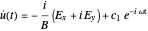 ,
,
where  is an arbitrary constant that can be determined by the initial condition
 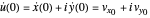 . In fact, this constant is
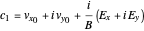 ,
,
so the solution is
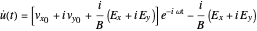 .
.
It is possible to decouple the equations in the  and
and  directions by introducing the constant
  that obeys

and
 .
.
This leads to
 ,
,
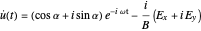
and using the relation  , we obtain

and then
 .
.
From the real part of this equation, we have
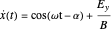
and from the imaginary part,
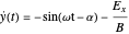 .
.
These equations can be solved by direct integration, which leads to

and
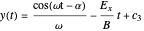 ,
,
where  and
and  are arbitrary constants. By the initial conditions
  and
and  , we obtain

and
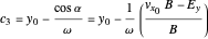 .
.
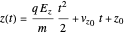
Using these constants and remembering that  , we obtain the final solutions
 ,
,
 ,
,
and
 .
.
Thus the problem is solved analytically, to give solutions that are plotted in 3D Cartesian coordinates.
Reference
[1] J. D. Jackson, Classical Electrodynamics, 3rd ed., New York: Wiley, 1999.
Permanent Citation
 Charged Particle Subjected to Lorentz Force
Deyvid W. M. Pastana, Vinicius B. Neves, Manuel E. Rodrigues and Luciano J. B. Quaresma Angular Distribution of Radiated Power Emitted by an Accelerated Point Charge
Deyvid W. M. Pastana, Manuel E. Rodrigues and Luciano J. B. Quaresma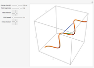 Charged Particle in a Uniform Magnetic Field
Jeff Bryant and Oleksandr Pavlyk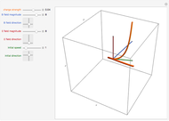 Charged Particle in Uniform Electric and Magnetic Fields
Jeff Bryant and Oleksandr Pavlyk Cycloidal Path of a Charged Particle in Uniform Perpendicular Electric and Magnetic Fields
Alexander Dalzell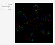 Dynamics of a Charged Particle in a Magnetic Field with a Kicked Electric Field
Enrique Zeleny Charged Particle in a Constant Electric Field Produced by Two Plates
Enrique Zeleny Motion of a Particle in Crossed Electric and Magnetic Fields
Ji?í Blecha Magnet Types in Particle Accelerators
Jakub Serych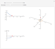 Proton Moving along the Axis of a Charged Ring
Enrique Zeleny