Chemical Equilibrium and Kinetics for HI Reaction


Requires a Wolfram Notebook System
Interact on desktop, mobile and cloud with the free Wolfram Player or other Wolfram Language products.
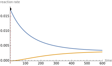
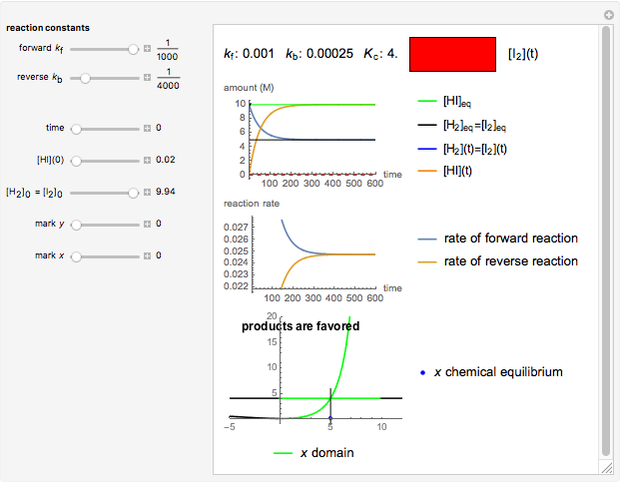
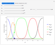
This Demonstration shows the effect of varying the rate constants  and
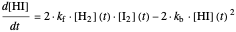
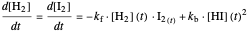
and  in a classic second-order chemical reaction
  .
.


Contributed by: S. Z. Lavagnino and D. Meliga (May 2016)
With additional contribution by: A. Chiavassa
Open content licensed under CC BY-NC-SA
Snapshots


Details
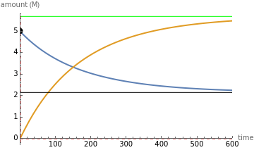
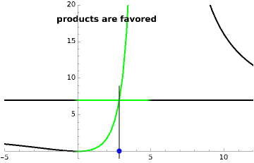
The final concentrations (green line for products, black line for reactants) have to be positive, but the value of  can be negative. There are three cases:
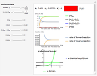
Snapshot 1: 
The position of the equilibrium is shifted to the right; the initial concentrations of the reactants  and
and  decrease, while the initial concentration of the product
  increases.
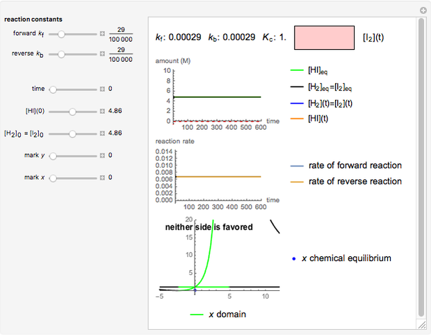
Snapshot 2: 
The reaction has already achieved the equilibrium status; macroscopically the initial concentrations of the reactants and the initial concentration of the product do not change.
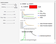
Snapshot 3: 
The position of the equilibrium is shifted to the left; the initial concentrations of the reactants increase, while the initial concentration of the product decreases.
The colored window represents the variation of  during the reaction because, as
  and
and  are colorless, the gaseous solution develops a reddish color depending on the concentration of
  , a typical color of this gas.
The marks  and
and  are guidelines to help assess the changes generated by the experimental conditions. Mark
  moves along the time axis (as in the first two plots), while mark
  is connected with the concentration axis of the first plot.
References
[1] G. Follo, S. Z. Lavagnino, and G. Valorio, "Scuola secondaria superiore (biennio): L'applicazione di DERIVE 5 alle tematiche inerenti l'equilibrio chimico," La Chimica nella Scuola, Rome: Aracne, 2015, pp. 31–44. www.aracneeditrice.it/pdf/9788854884328.pdf.
[2] D. A. McQuarrie and J. D. Simon, Chimica Fisica: Un approccio molecolare, Bologna: Zanichelli, 2000.
Permanent Citation
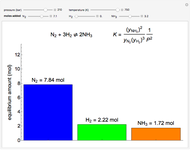 Chemical Equilibrium in the Haber Process
Benjamin L. Kee and Rachael L. Baumann Eyring-Polanyi versus Exponential Model for Chemical Reactions
Mark D. Normand, Christina S. Barsa, and Micha Peleg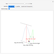 Kinetic and Thermodynamic Control of Electrophilic Addition Reactions
D. Meliga and S. Z. Lavagnino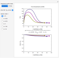 Extracting Fixed-Order Degradation Kinetics by the Endpoints Method
Mark D. Normand and Micha Peleg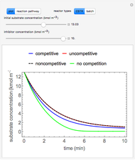 Inhibition of Enzyme Reactions in Continuous Stirred-Tank Reactor and Batch Reactor
Rachael L. Baumann Idealized Belousov-Zhabotinsky Reaction
Luca Zammataro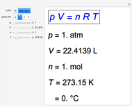 Ideal Gas Law Solver
S. M. Blinder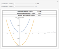 Marcus Theory of Electron-Transfer Reactions
Myles Lovasz, Nathan Tu, and Sherwin Navaz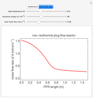 Parametric Sensitivity of Plug Flow Reactor With Heat Exchange
Rachael L. Baumann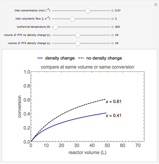 Why Density Change Cannot Be Ignored in a Plug Flow Reactor (PFR)
Rachael L. Baumann
-
 Crystal Field Theory for Coordination Complexes
D. Meliga -
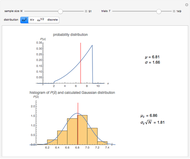 Central Limit Theorem Illustrated with Four Probability Distributions
D. Meliga -
Kinetic and Thermodynamic Control of Electrophilic Addition Reactions
D. Meliga -
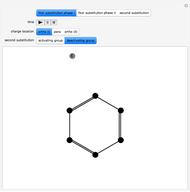 Electrophilic Aromatic Substitution Reactions of Benzene
D. Meliga -
 Electrophilic Addition to Alkenes with Formation of Optical Isomers
D. Meliga -
 Oil-Drop Experiment
D. Meliga -
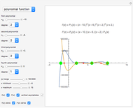 Zeros of a Polynomial or Rational Function and Its Derivative
D. Meliga -
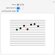
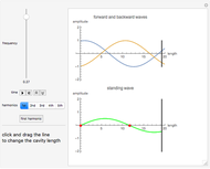 How to Catch a Standing Wave
D. Meliga -
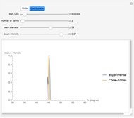 Comparing the Cook-Torrance BRDF Model with Diffuse Reflection Simulation
D. Meliga -
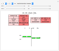 Stoichiometry: With Excess or Limiting Reagents
D. Meliga -
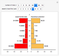 Dealer's Odds in Blackjack
D. Meliga -
 Rotating Crystal Method for 2D Lattices Using Ewald's Circle
D. Meliga -
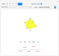
 Chemical Reactions Represented via a 3D Simplex
D. Meliga -
 Chemical Reactions Represented on a 2D Simplex
D. Meliga -
 Laue's Method for 2D Lattices Using Ewald's Circle
D. Meliga -
 Successive Dissociations of Polyprotic Acid H_4A as Regulated by pH
D. Meliga -
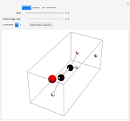
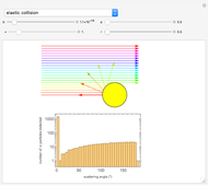 Detailed Analysis of Rutherford Scattering of Alpha Particles
D. Meliga -
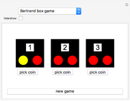 Bertrand's Box Paradox
D. Meliga -
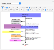 Classical Qualitative Inorganic Analysis
D. Meliga -
 Blood Donation Protocols
D. Meliga