Choosing Initial Parameter Values for Nonlinear Regression


Requires a Wolfram Notebook System
Interact on desktop, mobile and cloud with the free Wolfram Player or other Wolfram Language products.
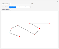
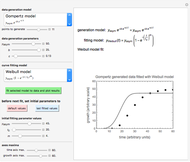
Fitting scattered experimental data with a multi-parameter model by nonlinear regression is frequently hampered by the difficulty in making sufficiently good guesses of the parameters' initial values. This Demonstration lets you plot the points from one of eight datasets and then use the model to generate a curve that approximately matches the data by manually adjusting the parameters’ values with sliders. The values that produce the visually matched curve are then used as the initial guesses to the regression procedure. The method is demonstrated with different scattered peaked datasets to be fitted with a double-stretched exponential model having four or five adjustable parameters. Hints: Start by matching  first. Try the Gradient method if Automatic frequently fails.
Contributed by: Mark D. Normand, Murray Eisenberg, and Micha Peleg (May 2012)
Open content licensed under CC BY-NC-SA
Snapshots


Details
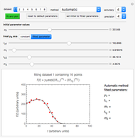
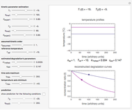
Snapshot 1: dataset 1 and corresponding curve after manually adjusting the parameters for successful completion of the regression using the Automatic method (five-parameter model where is to be fitted)
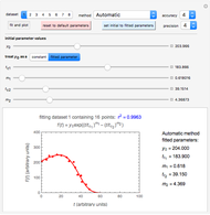
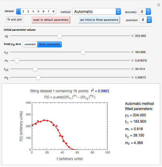
Snapshot 2: dataset 1 and corresponding curve after successful completion of the regression using the Automatic method (five-parameter model where is to be fitted)
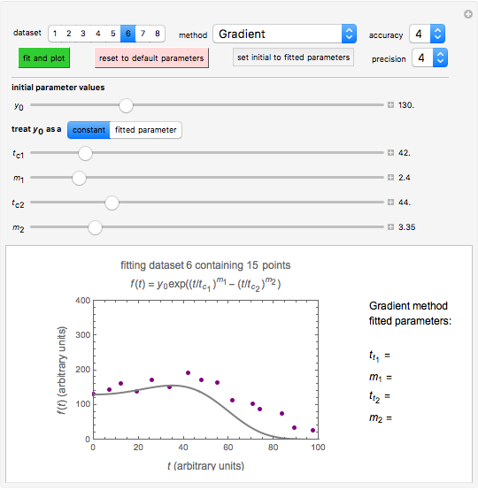
Snapshot 3: dataset 6 and corresponding curve after manually adjusting the parameters resulting in unsuccessful completion of the regression using the Gradient method (four-parameter model where is fixed)
Snapshot 4: dataset 6 and corresponding curve after manually adjusting the parameters for successful completion of the regression using the Gradient method (four-parameter model where is fixed)
Snapshot 5: dataset 6 and corresponding curve after successful completion of the regression using the Gradient method (four-parameter model where is fixed)
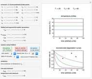
This Demonstration shows how scattered peaked data can be successfully fitted by nonlinear regression by finding initial guesses close enough to the parameters' actual values to yield a successful fit. You may choose any one of eight datasets and then attempt to match its plotted points with a curve using the model parameters’ sliders. The fitting model serving as an example is in the form of a double-stretched exponential  where
where  >
> . A setter bar is first used to choose between a four-parameter version of the model where is fixed as a constant and
  , ,
, ,  , and are adjustable parameters, and a five-parameter version where is also an adjustable parameter.
To start the procedure, select a dataset and click the "fit and plot" button. With the method set to Automatic the regression will fail with the default parameter values, and the message "Fit failed!" will be displayed in red above the plot. By adjusting the parameters’ sliders—always start by moving the slider until the curve passes through the first data point—try to match the curve to the data points and click on the "fit and plot" button again until successful, in which case the regression correlation coefficient,  , will be displayed in blue above the plot and the fitted parameter values will be shown to its left. Another option after failure is to change the method to Gradient. For these models and data sets the Gradient method is more likely to give a successful fit than Automatic. If both methods yield a successful fit, you should prefer the one giving the highest value. Additional controls let you change the regression's AccuracyGoal and PrecisionGoal.
After a successful fit, changing any control will erase the displayed and parameter values and signal that you are ready for a new fit attempt using the current slider settings as the parameters' initial values. To set the parameter sliders to the most recently fitted values, click the "set initial to fitted parameters" button. Click the "reset to default parameters" button to return the sliders to the original default parameter values.
An example of using this procedure with real experimental data can be found in [1].
Reference
[1] M. G. Corradini, M. D. Normand, M. Eisenberg, and M. Peleg, "Evaluation of a Stochastic Inactivation Model for Heat-Activated Spores of Bacillus spp.," Applied & Environmental Microbiology, 76, 2010 pp. 4402–4412.
Permanent Citation
 Global B-Spline Curve Interpolation
Shutao Tang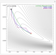 Iterations of Some Algorithms for Nonlinear Fitting
Heikki Ruskeepää Minimum Distance Explorer: Circle to Enclosed Polygon
Erik Mahieu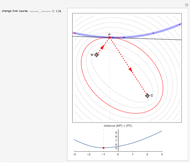 Lagrange's Milkmaid Problem
Erik Mahieu Shortest Path between Two Points on a Sphere
Bernard Vuilleumier Modeling a Simple Roller Coaster
Erik Mahieu Optimal Patch Exploitation
Nathan D. Dees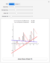 Ordinary Regression and Orthogonal Regression in the Plane
Tomas Garza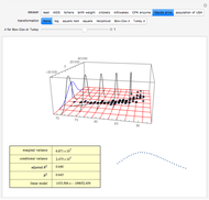 Regression Model with Transformations
Karl Heiner (SUNY at New Paltz) and Stan Wagon (Macalester College)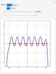 Seader's Method for Real Roots of a Nonlinear Equation
Housam Binous, Ahmed Bellagi, and Brian G. Higgins
-
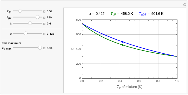 Gordon-Taylor and Fox Equations for Glass Transition Temperature
Micha Peleg -
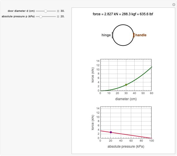 Force to Overcome Vacuum Pull
Micha Peleg -
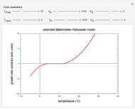 Extending the Square Root Growth Rate Model to Lethal Low Temperatures
Micha Peleg -
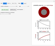 Probability of Being Strange According to Paulos
Micha Peleg -
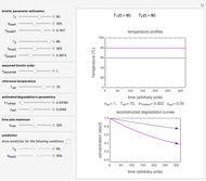
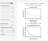 Successive Three-Point Method for Weibullian Chemical Degradation
Micha Peleg -
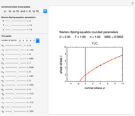 Estimating Cohesion and Tensile Strength of Compacted Powders
Micha Peleg -
 Three-Endpoints Method for Isothermal Weibullian Chemical Degradation
Micha Peleg -
 Vitamin C Loss in Foods During Heat Processing and Storage
Micha Peleg -
 Parameterizing Temperature-Viscosity Relations
Micha Peleg -
 Laplace Distribution in Fluctuating Stock Index Records
Micha Peleg -
 Weibullian Chemical Degradation
Micha Peleg -
 Simulating Ascorbic Acid Degradation
Micha Peleg -
 Additive and Multiplicative Risks
Micha Peleg -
 Endpoints Method for Predicting Chemical Degradation in Frozen Foods
Micha Peleg -
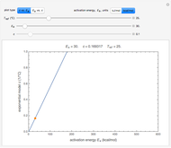 Exponential Model for Arrhenius Activation Energy
Micha Peleg -
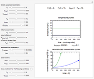
 Prediction of Isothermal Degradation by the Endpoints Method
Micha Peleg -
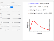 Risk Guesstimation from Factor Ranges
Micha Peleg -
 Volatiles Formation Kinetics in Stored Fish
Micha Peleg -
 Comparison of Six Sigmoid Growth Curve Models
Micha Peleg -
 Titration of Common Food Acids
Micha Peleg