Cobb-Douglas Utility Function


Requires a Wolfram Notebook System
Interact on desktop, mobile and cloud with the free Wolfram Player or other Wolfram Language products.
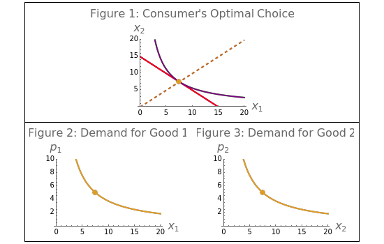
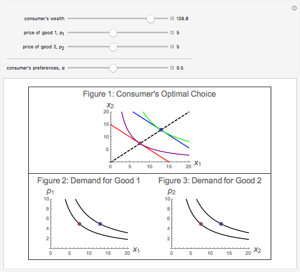
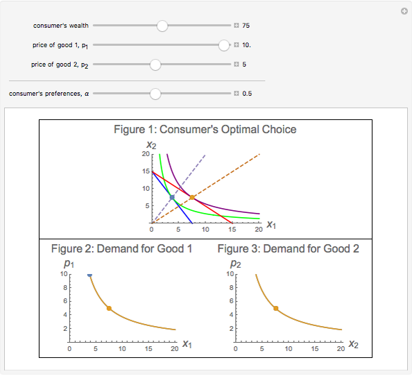
This Demonstration examines the Cobb–Douglas utility function. Figure 1 shows the consumer's optimal choice and wealth expansion paths. Figures 2 and 3 show demand curves. By modifying prices and wealth levels you can see how the consumer reacts to these changes. By modifying the parameter  (and holding prices and wealth fixed) you can compare the choices of two different consumers and the resulting demands.
Contributed by: Francisco José Espinosa (March 2011)
Open content licensed under CC BY-NC-SA
Snapshots


Details
Figure 1 depicts the optimal choice of a consumer whose preferences are represented by a Cobb–Douglas utility function. The purple indifference curve and the red budget line represent the initial situation ( and
and  ). By changing prices and wealth you can see how the consumer adjusts her decisions to the new environment. By leaving initial prices and wealth unchanged and modifying the parameter , you can see how two consumers with different preferences change from their optimal choices. In Figures 2 and 3, these changes in translate into changes in the consumer's willingness to pay for goods 1 and 2. (The effects always move in opposite direction: when willingness to pay for good 1 increases (falls), it falls (increases) for good 2.) From these figures you can also see that: (1) demands derived from a Cobb–Douglas utility function have no cross-price effects and (2) good 1 and good 2 are both normal goods for the consumer (and, because of this, both are also ordinary goods). Finally, you can notice that as long as the wealth level changes, optimal bundles are related by proportional expansion along rays from the origin.
Additional references:
Permanent Citation
 Optimization of Cobb-Douglas Function
Amir Ahmadi and Tom Creahan Constant Risk Aversion Utility Functions
Seth J. Chandler Land Use Regulation and Municipal Utility
Roger J. Brown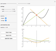 Elasticity Function
Timur Gareev An Example of a Production Function
Javier Puértolas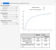 Terminal Wealth Optimization with Power and Log Utility
Daniel Michelbrink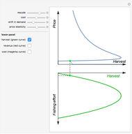 The Backward-Bending Supply Function in Fisheries
Arne Eide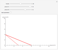 Changes in the Budget Line
Sarah Lichtblau Insurance Disclosures
Seth J. Chandler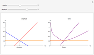 Profit Maximization in Perfect Competition
Fiona Maclachlan