Electromagnetic Waves from a Linear Antenna


Requires a Wolfram Notebook System
Interact on desktop, mobile and cloud with the free Wolfram Player or other Wolfram Language products.
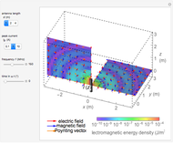
This Demonstration shows the electromagnetic fields around a linear antenna excited by a sinusoidal standing wave. The antenna direction is taken as the  axis. The electric and magnetic fields are displayed in the
  -
- and - planes together with Poynting vectors, shown by the arrows with length logarithmically scaled. The electromagnetic energy density is shown by color. You can vary the antenna length
  , current
  , and frequency
  , as well as the observation instant or phase
  . It is possible to see the animation by changing automatically, although you have to reduce the speed to a very low level.
Contributed by: Y. Shibuya (October 2013)
Open content licensed under CC BY-NC-SA
Snapshots


Details
The antenna current is assumed to be a standing wave  , where
  is the propagation constant (
 is the angular velocity and
  is the speed of light). From the charge conservation law, the charge density per unit length is
  . These complex values represent harmonic quantities. The scalar and vector potentials are determined by
 ,
,
 .
.
Using Mathematica's symbolic calculation in vector analysis, it is possible to write down the mathematical equations for the electromagnetic fields  and
and  in terms of
  and
and  directly. The somewhat lengthy expressions in the program are derived by approximating the integrations with the summations over the whole length of antenna parts (the number of divisions is set to eight for the sake of simplicity). The instantaneous fields are calculated by
  and
and  . Correspondingly, the Poynting vector is calculated by
  , and the electromagnetic energy density by
  .
.
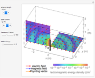
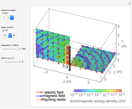
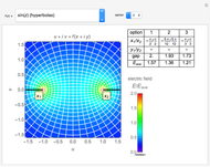
Denoting the wavelength  by
by  , snapshots 1, 2, and 3 are cases for
  , , and
  , respectively. In the first two cases, the electromagnetic radiation is directed laterally, but in the relatively long antenna for snapshot 3, substantial radiation is produced near the axial directions.
Reference
[1] J. D. Jackson, Classical Electrodynamics, 3rd ed., New York: John Wiley & Sons, 1998.
Permanent Citation
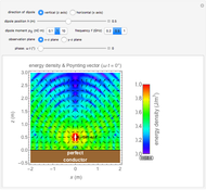 Electromagnetic Wave from Dipole over a Perfect Conductor
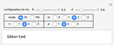
Y. Shibuya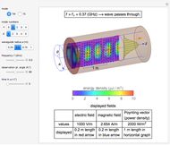 Electromagnetic Waves in a Cylindrical Waveguide
Y. Shibuya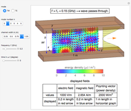 Electromagnetic Waves in a Parallel-Plate Waveguide
Y. Shibuya Electromagnetic Wave Incident on a Perfect Conductor
Y. Shibuya Electromagnetic Wave Incident on a Dielectric Boundary
Y. Shibuya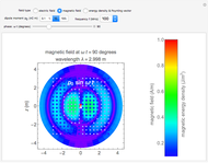 Electromagnetic Fields For Hertzian Dipoles
Y. Shibuya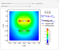 Electromagnetic Fields in Wireless Power Transmission
Y. Shibuya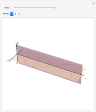 Electromagnetic Wave
Enrique Zeleny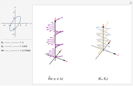 Polarization of an Electromagnetic Wave
Luis Jonathan Cervantes Rosas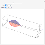 Propagation of a Plane Electromagnetic Wave
Alan Fafard
-
 Skin Effects in Straight Wires
Y. Shibuya -
 Leakage Inductance in a Transformer
Y. Shibuya -
 Electromagnetic Wave Scattering by Conducting Sphere
Y. Shibuya -
 Cylindrical Cavity Resonator
Y. Shibuya -
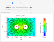 Electric Fields for Pairs of Cylinders or Spheres
Y. Shibuya -
Electromagnetic Fields in Wireless Power Transmission
Y. Shibuya -
 Wireless Power Transmission
Y. Shibuya -
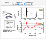
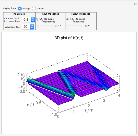 Surge Propagation in a Transmission Line
Y. Shibuya -
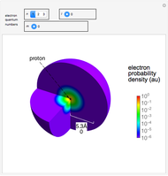 Electron Probability Distribution for the Hydrogen Atom
Y. Shibuya -
 Magnetic Shielding Effect of a Spherical Shell
Y. Shibuya -
 Electromagnetic Waves from a Linear Antenna
Y. Shibuya -
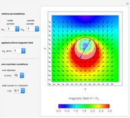 Current-Carrying Wire in Uniform Magnetic Field
Y. Shibuya -
Electromagnetic Wave Incident on a Dielectric Boundary
Y. Shibuya -
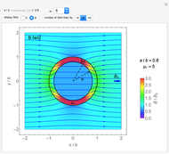
 Magnetic Field and Magnetic Induction in a Cylindrical Bar Magnet
Y. Shibuya -
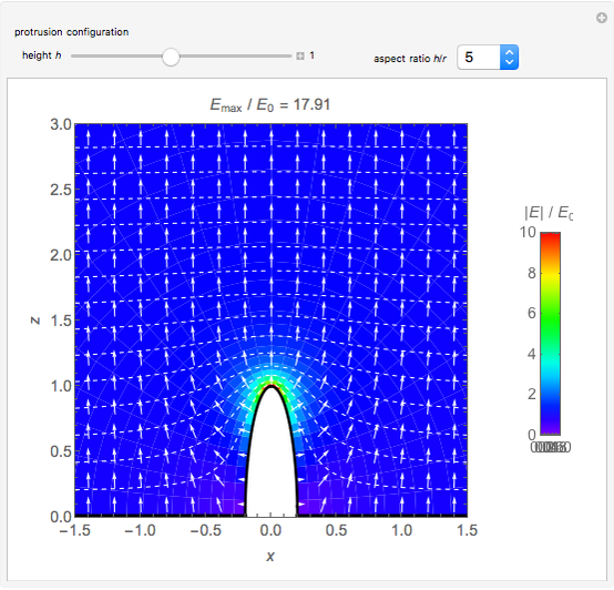 Spheroidal Protrusion in a Uniform Electric Field
Y. Shibuya -
 Electrostatic Fields Using Conformal Mapping
Y. Shibuya -
 Dielectric Sphere in a Uniform Electric Field
Y. Shibuya -
 Electromagnetic Waves in Optical Fibers
Y. Shibuya -
Electromagnetic Waves in a Cylindrical Waveguide
Y. Shibuya -
Electromagnetic Waves in a Parallel-Plate Waveguide
Y. Shibuya