European Binomial Option Pricing with Nonconstant Volatility

Requires a Wolfram Notebook System
Interact on desktop, mobile and cloud with the free Wolfram Player or other Wolfram Language products.
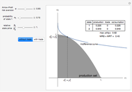
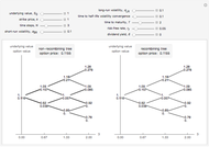
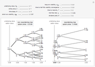
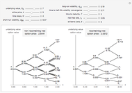
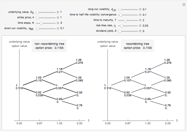
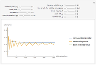
This Demonstration shows two approaches to using binomial option pricing for a European call option on an underlying asset with nonconstant volatility. The holder of the option has the right but not the obligation to purchase an asset at some fixed maturity date  in the future for a price agreed upon today (known as the strike price
  ).
).


Contributed by: Tom Stannard and Graeme Guthrie (June 2015)
Open content licensed under CC BY-NC-SA
Snapshots

Details
In [2], Guthrie presents a real options model where an investor is deciding whether or not to invest in a project. At time the option to invest expires. The investor begins with some level of uncertainty of the project's true value  . Each period the investor receives a signal
 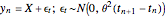 and uses this signal to update their perception of the investment's true value
  from
from  to
to  ;
;  is a constant that determines the amount of noise in each signal. High means each signal is noisy and the investor cannot update their perception very much ( and
  are inversely related). The initial uncertainty of the true value is
  , and after each signal this is also updated and decreased to
  to reflect that more information about the project has been revealed;
  is the volatility of the market (that will become the long-term volatility). The volatility at each time step
  for this learning process is
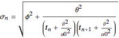 .
.
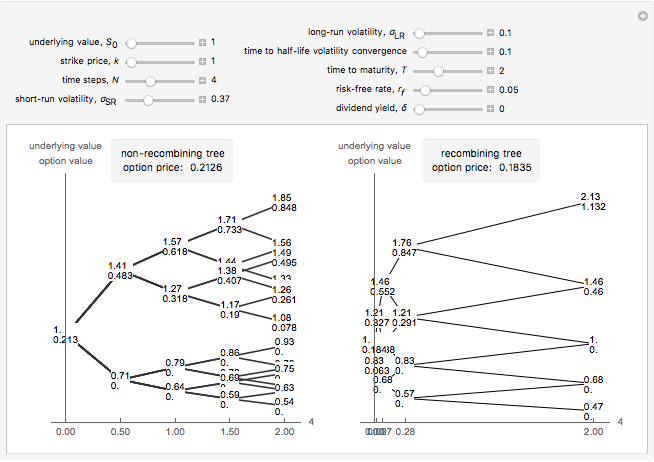
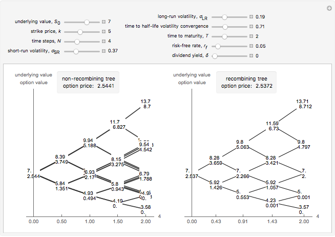
If we use this for constant-sized time steps (constant  ), then we get the non-recombining case. This is because the noise term and the residual uncertainty make the volatility decrease over time. That is, early information is more revealing than later information about the project's true value. [2] presents an alternative approach where constant movements can be calculated by
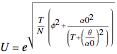
subject to time steps calculated using
 .
.
In order to apply this to an option on an asset, we can replace the initial uncertainty with a share price at the inception of the contract  . We then specify as the long-term volatility of the asset and calculate short- and long-run volatility along with the time to half-life convergence of the two to calculate and as
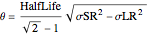 ,
,
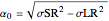 .
.
These values can then be placed into the equations for ,  , and
, and  , and the models in the Demonstration can be built.
References
[1] J. Cox, S. Ross, M. Rubinstein, "Option Pricing: A Simplified Approach," Journal of Financial Economics, 7(3), 1979 pp. 229–263. doi:10.1016/0304-405X(79)90015-1.
[2] G. Guthrie, "Learning Options and Binomial Trees," Wilmott Journal: The International Journal of Innovative Quantitative Finance Research, 3(1), 2011 pp. 1–23. doi:10.1002/wilj.42.
[3] J. C. Hull, Options, Futures, and Other Derivatives, 8th ed., Boston: Prentice Hall, 2012.
Permanent Citation
 Convergence of Binomial Option Pricing under Nonconstant Volatility
Tom Stannard Binomial Option Pricing Model
Fiona Maclachlan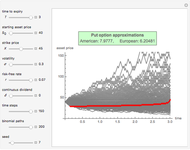 Pricing Put Options with the Binomial Method
Michail Bozoudis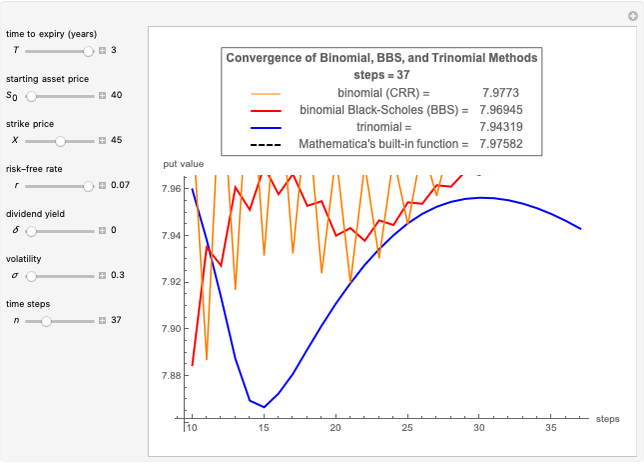 Convergence of Binomial, Binomial Black-Scholes, and Trinomial Option Pricing Methods
Michail Bozoudis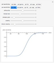 European Option Greeks
Michael Kelly (Stuart GSB, Illinois Institute of Technology)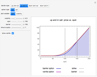 Barrier Option Pricing within the Black-Scholes Model
Peter Falloon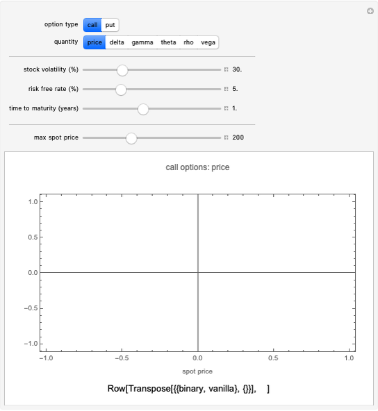 Binary Options: Pricing and Greeks
Peter Falloon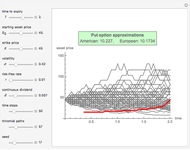 Pricing Put Options with the Trinomial Method
Michail Bozoudis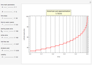 A Recursive Integration Method for Options Pricing
Michail Bozoudis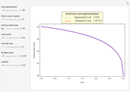 Kim's Method for Pricing American Options
Michail Bozoudis