Grover's Quantum Search Algorithm

Requires a Wolfram Notebook System
Interact on desktop, mobile and cloud with the free Wolfram Player or other Wolfram Language products.
Quantum computers may solve some problems dramatically faster than conventional machines. One example is searching an unordered set for an item with specific properties. A quantum algorithm can find such an item (a "solution") in a time proportional to the square root of the size of the set, which is considerably faster than conventional ("classical") methods on large sets.
[more]
Contributed by: Tad Hogg (March 2011)
Open content licensed under CC BY-NC-SA
Snapshots


Details
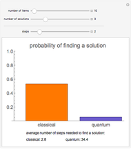
Snapshot 1: With one solution out of 10 items, four steps of the quantum algorithm give less chance for a solution than two steps, showing the quantum algorithm can perform worse with more steps.
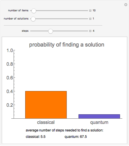
Snapshot 2: With three solutions out of 10 items, two steps of the quantum algorithm give a small chance of finding a solution, showing the best number of steps depends on the number of solutions.
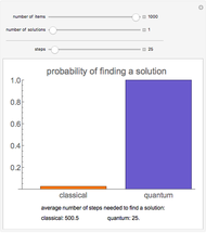
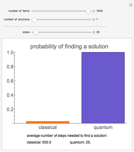
Snapshot 3: With one solution out of 1000 items, the quantum algorithm performs well with just 25 steps, which is much better than the classical method.
The search problem in this Demonstration is unstructured, that is, each item only provides a single bit of information: whether it is a solution or not. Thus, the nonsolution items provide no information on where else to find a solution. This lack of information makes solutions difficult to find when there are many items but few solutions. This Demonstration shows the behavior of the best classical and quantum algorithms for an unstructured search.
The controls number of items and number of solutions set the difficulty of the problem by changing the size of the set and the number of solutions. The text below the plot shows the average number of steps required for each algorithm to find a solution.
The classical algorithm is generate-and-test, that is, examine items one at a time until a solution is found. When the set has  items, of which
  are solutions, the probability of finding a solution increases monotonically with the number of items examined until, after
  steps, a solution is guaranteed to be found. The classical algorithm stops as soon as it finds a solution. On average, the algorithm finds a solution after
  steps.
In the quantum algorithm, due to Lov Grover, the probability of finding a solution is close to 1 when the number of steps is about  . So the average number of steps in finding a solution is proportional to
  , much less than the linear growth with for the classical algorithm. The quantum algorithm gives no answer until it completes the prespecified number of steps, and must restart from the beginning if it does not find a solution. Each repetition adds to the total number of steps required by the algorithm. Thus, if
  is the probability of finding a solution when run for a given number of steps, the average number of steps required to find a solution, including any repetitions, is
  .
.
The probability for the quantum algorithm to find a solution oscillates with the number of steps. So taking more steps than needed to reach probability near 1 decreases the chance of finding a solution. Thus, the quantum algorithm requires care in selecting the number of steps. For example, a certain number of steps could find a solution with high probability when there is just one solution, but have only a small chance of finding a solution when there are, say, two or three solutions.
This Demonstration compares the algorithms' performance in terms of the number of steps to find a solution. There are several caveats in relating this comparison to practical performance. First, the comparison is just for algorithm operation, and does not account for creating the set in a form suitable for the algorithms' use. Second, to compare actual runtime, the number of steps must be multiplied by the time for each step. Due to physical implementation challenges and extensive error correction, quantum computers will likely run with a slower clock rate than conventional machines. Thus, each step will take longer on a quantum computer, somewhat reducing the advantage of using fewer steps. Finally, physical implementation of the quantum method in terms of two-state quantum systems (called "qubits") is simplest when the number of items is a power of two. For simplicity, this Demonstration does not make this restriction on the number of items.
See L. Grover, "Quantum Mechanics Helps in Searching for a Needle in a Haystack," Physical Review Letters, 79(2), 1997 pp. 325–328 for a discussion of the algorithm and a proof of its performance with a single solution.
If the number of solutions is not known, repeating the algorithm with an increasing number of steps whenever a solution is not found maintains the good performance of this method. For a description of this method, see M. Boyer, G. Brassard, P. Hoyer, and A. Tapp, "Tight Bounds on Quantum Searching," Fortschritte der Physik, 46(4–5), 1998 pp. 493–506.
If the set of items has some structure, that is, properties of nonsolution items give some indication of where solutions are located, then other algorithms, both classical and quantum, can often exploit the structure to find a solution much faster than unstructured search algorithms. The alphabetical ordering of a dictionary is an example of such structure, which allows finding a given word's definition much more rapidly than the unstructured search algorithms shown in this Demonstration.
Permanent Citation
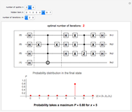 Quantum Circuit Implementing Grover's Search Algorithm
Alexander Prokopenya Quantum Computer Search Algorithms
Tad Hogg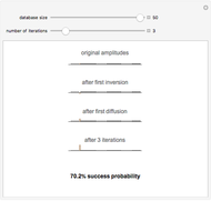 Simulated Quantum Computer Algorithm for Database Searching
S. M. Blinder Bubble Sort Algorithm
Enrique Zeleny Markov Chain Monte Carlo Simulation Using the Metropolis Algorithm
Philip Gregory (Physics and Astronomy, University of British Columbia) Brute-Force String Matching
Michael Schreiber Comparing Sorting Algorithms on Rainbow-Colored Bar Charts
Michael Zhou and Karolina Urban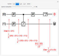 Deutsch's Algorithm on a Quantum Computer
S. M. Blinder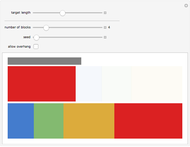 Optimal Bin Packing with Random Lengths
Yifan Hu and Stephen Wolfram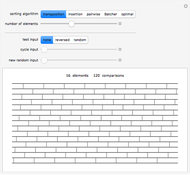 Sorting Networks
Stephen Wolfram
-
 Compressing Ideal Fermi and Bose Gases at Low Temperatures
Tad Hogg -
 Irreversible and Reversible Temperature Equilibration
Tad Hogg -
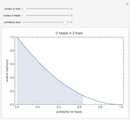 Maximum Likelihood Estimation for Coin Tosses
Tad Hogg -
 Stroop Effect: Reading Colored Words
Tad Hogg -
 Bijective Mapping of an Interval to a Square
Tad Hogg -
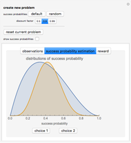 The Multi-Arm Bandit
Tad Hogg -
 Juggling the Cascade Pattern
Tad Hogg -
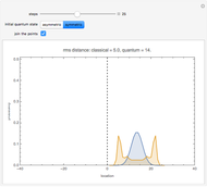 Quantum Random Walk
Tad Hogg -
 Diffusion to a Spherical Reactor
Tad Hogg -
 Particles Thrown from a Rotating Bar
Tad Hogg -
 Grover's Quantum Search Algorithm
Tad Hogg -
Simulated Quantum Computer Algorithm for Database Searching
Tad Hogg -
Quantum Computer Search Algorithms
Tad Hogg