How Continuous Innovation Affects Supply, Producer Surplus, and Consumer Surplus


Requires a Wolfram Notebook System
Interact on desktop, mobile and cloud with the free Wolfram Player or other Wolfram Language products.
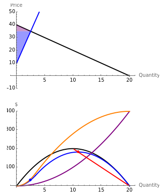
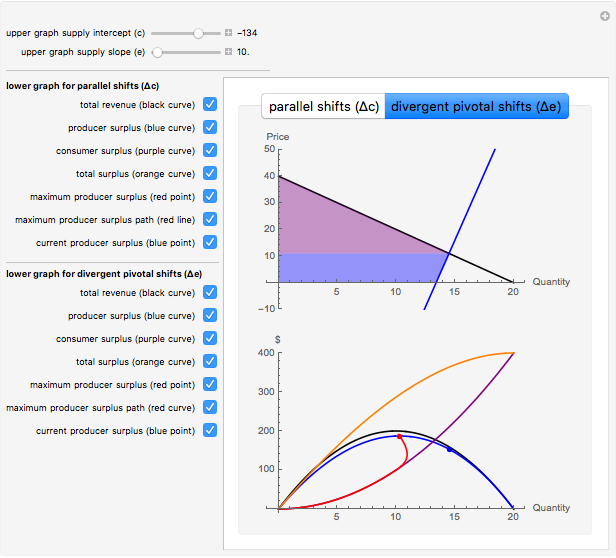
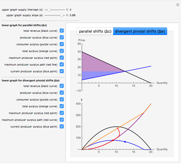
This Demonstration shows producer surplus (PS), consumer surplus (CS), and total surplus (TS) when there are parallel shifts in supply  and divergent pivotal shifts in supply
  . Innovations that favor low-productivity/high-cost producers create divergent pivotal shifts in supply, which can be simulated by increasing the slope of the supply curve
  while keeping the
  intercept
  constant. On the other hand, innovations that create similar benefits to both the high-productivity/low-cost producers and low-productivity/high-cost producers create parallel shifts in supply. Rightward parallel shifts in supply can be simulated by decreasing the intercept of the supply curve while keeping the slope constant.


Contributed by: John B. Horowitz, Michael A. Karls, Juan Sesmero, and T. Norman Van Cott (May 2015)
The idea for labeling curves and shading regions is based on code from "Consumer and Producer Surplus" by Fiona Maclachlan.
The idea for selecting curves to display via checkboxes is based on code from "The Backward-Bending Supply Function in Fisheries" by Arne Eide.
Open content licensed under CC BY-NC-SA
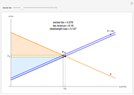
Snapshots


Details
Reference
[1] J. B. Horowitz, M. A. Karls, J. Sesmero, and T. N. Van Cott. "Teaching Students How Continuous Innovation Affects Supply, Producer Surplus, and Consumer Surplus." Ball State University Department of Economics Working Paper Series, ECWP201415, 2015. cms.bsu.edu/academics/collegesanddepartments/mcob/majors-and-degrees/depts/economics/facultyresearch/workingpaperseries.
Permanent Citation
 Supply and Demand Excise Tax
Nicholas Palmer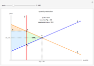 Supply and Demand Quantity Restriction
Nicholas Palmer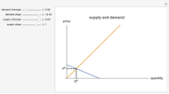 Basic Supply and Demand
Mark Gillis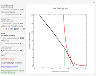 Two-Period Consumer Model with Different Interest Rates
Andres F. Rodriguez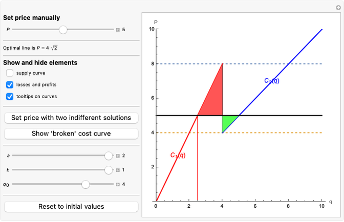 Supply Curve from Piecewise Linear Cost Function
Timur Gareev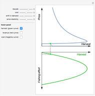 The Backward-Bending Supply Function in Fisheries
Arne Eide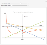 No Supply Curve in a Monopolistic Market
Samuel G. Chen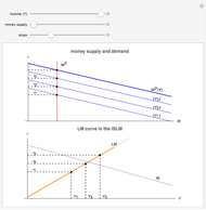 Deriving the Liquidity Preference-Money Supply (LM) Curve
Nicholas Palmer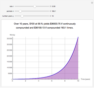 Continuous versus Compounded Interest
Jonathan Scherzer and Yossi Quint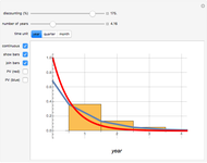 Continuous and Discrete Time Discounting
Arne Eide
