Karush-Kuhn-Tucker (KKT) Conditions for Nonlinear Programming with Inequality Constraints


Requires a Wolfram Notebook System
Interact on desktop, mobile and cloud with the free Wolfram Player or other Wolfram Language products.
This Demonstration explores a constrained nonlinear program in which the objective is to minimize a function  subject to a single inequality constraint
  . The top-left box shows the level sets of
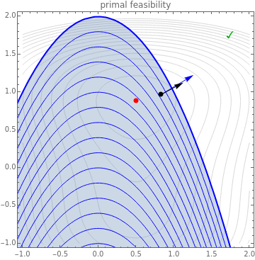
  as gray contours, the level sets of
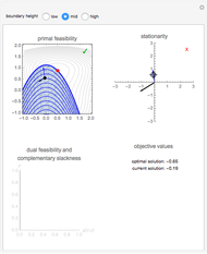
  as blue contours and the feasible region as a shaded blue area. The optimal feasible solution is shown as a red dot. Clicking anywhere inside the top-left box selects a point as a candidate solution; the radio buttons adjust the location of the feasible region. All three boxes display visual representations of the Karush–Kuhn–Tucker conditions, along with a green checkmark or a red Χ to indicate that the candidate does or does not satisfy the condition, respectively. In particular, the top two boxes display
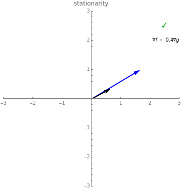
  as a black arrow and
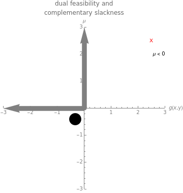
  as a blue arrow, while the bottom left box displays a point corresponding to the KKT multiplier
  (provided it exists, which requires that either
  or that and are collinear) and the value of . In order for a solution to be the gobal optimum, it is necessary to satisfy all of the conditions simultaneously.
Contributed by: Adam Rumpf (July 2018)
Open content licensed under CC BY-NC-SA
Snapshots


Details
The Karush–Kuhn–Tucker conditions (a.k.a. KKT conditions or Kuhn–Tucker conditions) are a set of necessary conditions for a solution of a constrained nonlinear program to be optimal [1]. The KKT conditions generalize the method of Lagrange multipliers for nonlinear programs with equality constraints, allowing for both equalities and inequalities. In this Demonstration, we consider only inequality constraints. Specifically, the problem used for this Demonstration has the form

such that
where and are both real-valued, differentiable functions on  that satisfy the regularity conditions needed for the KKT conditions to apply [2]. For this simple problem, the KKT conditions state that a solution
  is a local optimum if and only if there exists a constant (called a KKT multiplier) such that the following four conditions hold:
1. Stationarity: 
2. Primal feasibility: 
3. Dual feasibility: 
4. Complementary slackness: 
There are two possibilities for the optimal solution: it can occur either on the boundary of the feasible set (where  ) or on the interior (where
  ). If it occurs on the boundary, then we are left with the equivalent of an equality constraint, in which case the simple method of Lagrange multipliers applies. The preceding stationarity condition is identical to the one for Lagrange multipliers, and it captures instances for which either (meaning that becomes flat on the boundary) or
  (meaning that the level sets of and lie tangent to each other). The first case forces
  , while the second forces
  .
.
If, on the other hand, the optimum occurs on the interior, then the constraint has no effect on the calculation of the optimum. This can only occur where , but the stationarity condition guarantees simply that at least one out of and is true, with no guarantees about which one holds. Additional conditions are needed to ensure that for any candidate optimum on the interior. The snapshots include various examples of solutions that are not locally optimal and satisfy some (but not all) of the KKT conditions.
Dual feasibility ensures that the optimum occurs on the correct side of the feasible boundary by ensuring that and point in opposite directions. Complementary slackness ensures that the correct restriction is enforced. The condition itself forces at least one of and to vanish. On the interior of the feasible set, we have , in which case complementary slackness enforces and thus . On the boundary, we have , in which case is unrestricted.
The three boxes contained in this Demonstration graphically illustrate each of these conditions. Primal feasibility is satisfied exactly when the chosen point lies inside the feasible region. The top two boxes of the Demonstration display as a black arrow and as a blue arrow. The bottom-left box shows a point on the versus axis corresponding to the current values of and . The positive and negative axes are highlighted to indicate the coordinates that simultaneously satisfy dual feasibility and complementary slackness. Note that is only defined when or when and are collinear, and that no point is plotted when does not exist.
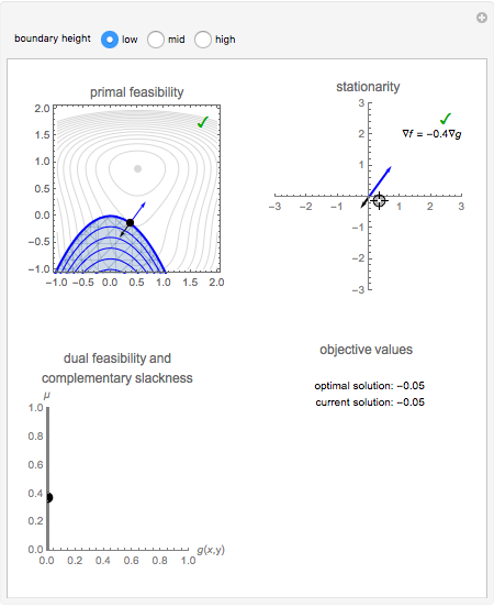
Snapshot 1: an optimal solution on the boundary of the feasible region. Here we do not have , so the optimal solution is a stationary point on the boundary. Note that (the black arrow) and (the blue arrow) point in opposite directions. In this case, we have  and ; therefore, dual feasibility and complementary slackness are also satisfied.
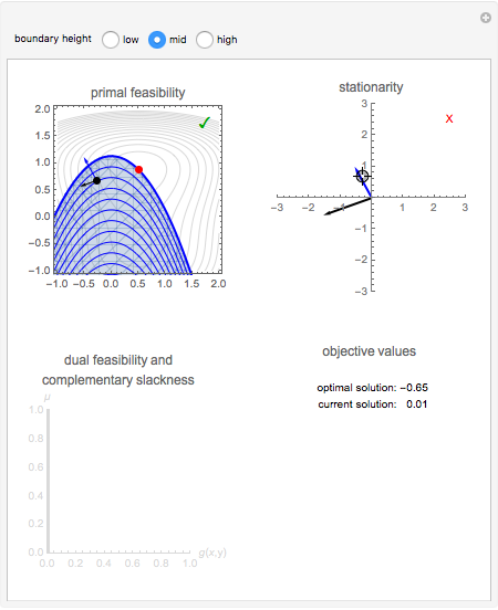
Snapshot 2: a clearly nonoptimal solution on the interior of the feasible region. Stationarity is not satisfied, therefore there exists no value such that  . With no KKT multiplier, dual feasibility and complementary slackness are meaningless, and so there is nothing to report in the bottom-left box.
Snapshot 3: a nonoptimal solution that does not satisfy complementary slackness. This means that (so  ) and
) and  (so we are not on the boundary), which contradicts the only possible interior solutions coinciding with being flat.
Snapshot 4: a nonoptimal solution that satisfies only stationarity. This indicates that if the level sets of were extended outside of the feasible region, then one would lie tangent to a level set of at this point, but the point is obviously not feasible.
Snapshot 5: an optimal solution inside the feasible region. As is necessary for such a solution, we have .
Snapshot 6: a nonoptimal solution that does not satisfy dual feasibility. This is identical to the example from Snapshot 5, but the point has been shifted to the right and away from where is flat. Here and point in the same direction and  , which indicates that moving further toward the interior would decrease ; therefore, the current solution cannot be optimal.
References
[1] D. P. Bertsekas, Nonlinear Programming (2nd ed.), Belmont, MA: Athena Scientific, 1999.
[2] R. G. Eustáquio, E. W. Karas and A. A. Ribeiro, Constraint Qualifications for Nonlinear Programming, Working paper, Department of Mathematics, Federal University of Paraná, Brazil, 2007. www.researchgate.net/publication/230663810_Constraint _Qualifications _for _Nonlinear _Programming.
Permanent Citation
 Affine-Scaling Interior Point Method
Andreas Lauschke Two-Phase Simplex Method
Sourav Mukherjee Parametric Linear Programming
Bunduchi Ecaterina and Mandric Igor 0-1 Knapsack Problem
Conrad A. Benulis Stage Illumination Problem
Slobodan Jelic and Domagoj Matijevic Computable General Equilibrium (CGE) of Multiregion Input-Output Model
Stuart Nettleton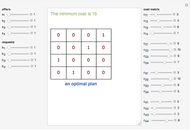 Monge-Kantorovich Transportation Problem
Mandric Igor (Moldova State University)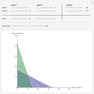 A Simple, Standard Linear Programming Scenario
Chris Boucher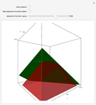 Graphical Linear Programming for Three Variables
Olivia M. Carducci (East Stroudsburg University)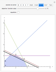 Graphical Linear Programming for Two Variables
Olivia M. Carducci (East Stroudsburg University)
-
 Karush-Kuhn-Tucker (KKT) Conditions for Nonlinear Programming with Inequality Constraints
Adam Rumpf -
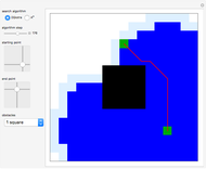 Dijkstra's and A* Search Algorithms for Pathfinding with Obstacles
Adam Rumpf -
 Comparing Voting Systems for a Normal Distribution of Voters
Adam Rumpf -
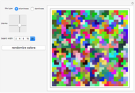 Domino and Triomino Tilings of a Chessboard
Adam Rumpf -
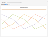 Tracing Card Paths during Perfect Shuffles
Adam Rumpf -
 Animated Remainder Graph
Adam Rumpf