Loading Plot of a Principal Component Analysis (PCA)


Requires a Wolfram Notebook System
Interact on desktop, mobile and cloud with the free Wolfram Player or other Wolfram Language products.
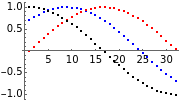
Principal component analysis (PCA) is a statistical procedure that converts data with possibly correlated variables into a set of linearly uncorrelated variables, analogous to a principal-axis transformation in mechanics.
[more]
Contributed by: D. Meliga and S. Z. Lavagnino (May 2016)
With additional contributions by: A. Chiavassaand M. Aria
Open content licensed under CC BY-NC-SA
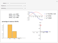
Snapshots


Details
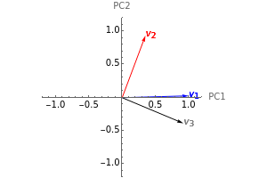
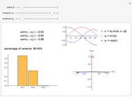
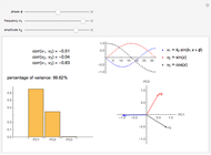
In the loading plot, the high correlation between two variables leads to two vectors that are very close to each other, the non-correlation leads to two vectors out of phase by  , while the anti-correlation leads to two vectors that are out of phase by
  [2].
[2].
Snapshot 1: a strong correlation between  and
and 
 , non-correlation in the remaining cases
  . From a graphical point of view, we can see two vectors that are very close, while the others are out of phase with each other by about .
Snapshot 2: a strong correlation between and 
 , non-correlation in the remaining cases . From a graphical point of view, we can see two opposite vectors, while the others are out of phase to each other by about .
References
[1] S. J. Press, Applied Multivariate Analysis: Using Bayesian and Frequentist Methods of Inference, Mineola, NY: Dover Publications, 2005.
[2] M. Aria. "L'analisi in Componenti Principali." (May 25, 2016) www.federica.unina.it/economia/analisi-statistica-sociologica/analisi-componenti-principali.
Permanent Citation
 Aliasing in Time Series Analysis
Ian McLeod 1, 2, 3-Parameter Logistic Rasch and Birnbaum Models and Item Analysis
Olexandr Eugene Prokopchenko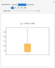 Exploring Skewness in Box Plots
Ian McLeod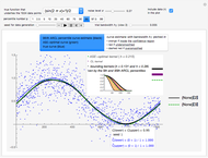 Nonparametric Regression and Kernel Smoothing: Confidence Regions for the L2-Optimal Curve Estimate
Didier A. Girard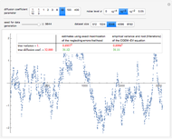 Estimating a Centered Ornstein-Uhlenbeck Process under Measurement Errors
Didier A. Girard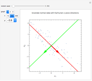 Principal Components
Ian McLeod Fisher Discriminant Analysis
Ian McLeod Cluster Analysis for 2D Points
Stephen Wolfram Edgeworth Expansion for Near-Normal Data
Housam Binous, Mamdouh Al-Harthi, and Brian G. Higgins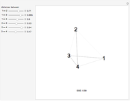 Multidimensional Scaling
Yaroslav Bulatov
-
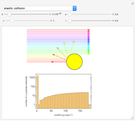
 Single-Step Reaction Kinetics Using Collision Theory
S. Z. Lavagnino -
 Crystal Field Theory for Coordination Complexes
S. Z. Lavagnino -
 Central Limit Theorem Illustrated with Four Probability Distributions
S. Z. Lavagnino -
 Kinetic and Thermodynamic Control of Electrophilic Addition Reactions
S. Z. Lavagnino -
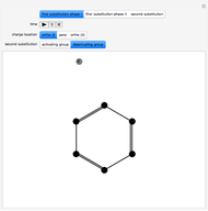 Electrophilic Aromatic Substitution Reactions of Benzene
S. Z. Lavagnino -
 Electrophilic Addition to Alkenes with Formation of Optical Isomers
S. Z. Lavagnino -
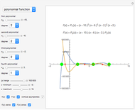 Zeros of a Polynomial or Rational Function and Its Derivative
S. Z. Lavagnino -
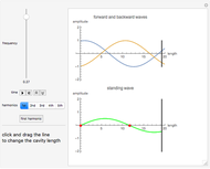 How to Catch a Standing Wave
S. Z. Lavagnino -
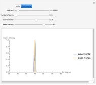 Comparing the Cook-Torrance BRDF Model with Diffuse Reflection Simulation
S. Z. Lavagnino -
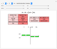 Stoichiometry: With Excess or Limiting Reagents
S. Z. Lavagnino -
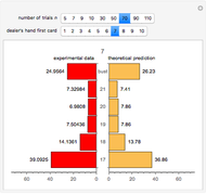 Dealer's Odds in Blackjack
S. Z. Lavagnino -
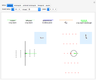 Rotating Crystal Method for 2D Lattices Using Ewald's Circle
S. Z. Lavagnino -
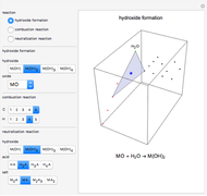 Chemical Reactions Represented via a 3D Simplex
S. Z. Lavagnino -
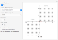 Chemical Reactions Represented on a 2D Simplex
S. Z. Lavagnino -
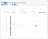 Laue's Method for 2D Lattices Using Ewald's Circle
S. Z. Lavagnino -
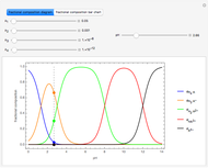 Successive Dissociations of Polyprotic Acid H_4A as Regulated by pH
S. Z. Lavagnino -
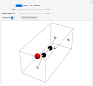
 Detailed Analysis of Rutherford Scattering of Alpha Particles
S. Z. Lavagnino -
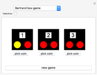 Bertrand's Box Paradox
S. Z. Lavagnino -
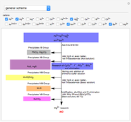 Classical Qualitative Inorganic Analysis
S. Z. Lavagnino -
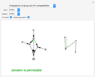 Blood Donation Protocols
S. Z. Lavagnino