Local Regression for Country Data

Requires a Wolfram Notebook System
Interact on desktop, mobile and cloud with the free Wolfram Player or other Wolfram Language products.
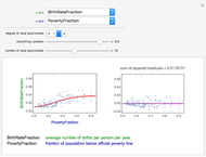
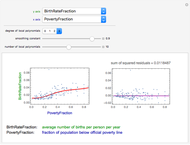
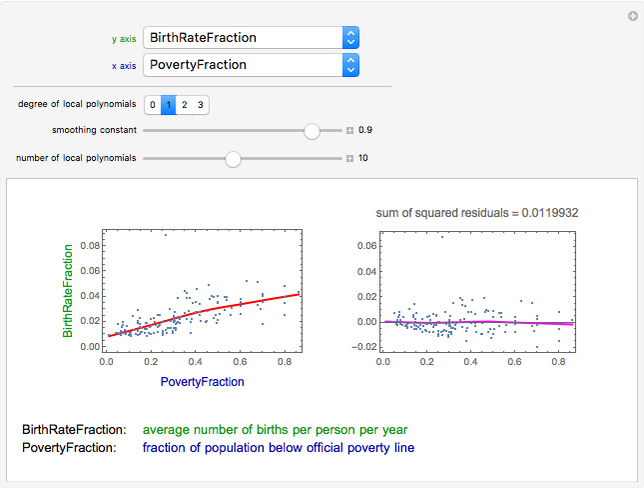
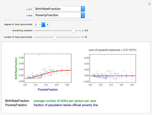
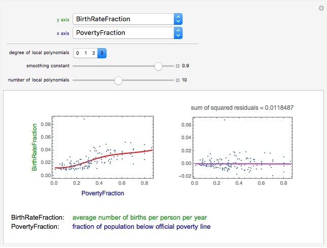
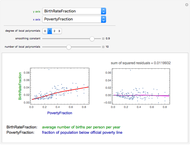
This Demonstration studies pairwise relationships between properties of countries. A total of 124 properties can be studied. The figure on the left gives the scatter plot of the points. It also gives a local regression curve that is calculated with the so-called loess method [1]. The local regression curve describes the trend of the data, thus giving a guide to infer the nature of the relationship between the two properties. The figure on the right gives the residuals of the regression together with a local regression curve to the residuals. This figure gives information about the quality of the local regression curve shown in the left figure: the closer the local regression curve of the residuals is to zero, the better the local regression curve fits the data.
Contributed by: Heikki Ruskeepää (March 2010)
After work by: Stephen Wolfram
Open content licensed under CC BY-NC-SA
Snapshots
Details
Snapshot 1: degree = 1, smoothing = 0.9: residuals could be somewhat closer to zero
Snapshot 2: degree = 2, smoothing = 0.9: residuals are quite close to zero and the fit is good
Snapshot 3: degree = 3, smoothing = 0.9: residuals are close to zero but the curve seems to be an overfit
Snapshot 4: degree = 1, smoothing = 0.1: residuals are close to zero but the fit is not smooth
Snapshot 5: degree = 1, smoothing = 0.6: residuals are close to zero and the fit is smooth; good settings
Snapshot 6: degree = 1, smoothing = 1.0: residuals are not close enough to zero
Snapshot 7: degree = 2, number of polynomials = 10: not a good fit
Snapshot 8: degree = 0, number of polynomials = 10: a reasonable fit
Snapshot 9: degree = 1, number of polynomials = 2: another reasonable fit
The points in a scatter plot often form a group that does not have a very clear form, so that choosing a suitable degree for a usual polynomial regression curve may be difficult. A local regression curve may then be a solution. Such a curve studies the data locally at many points and the result may be quite a good description of the trend in the data. One of the local regression methods is loess (LOcal regrESSion) (see [1, pp. 91–101]), and we use this method. For Mathematica code for loess, see [2, pp. 1038–1041].
In loess, we choose a set of points from the range of the independent variable and fit a set of low-order polynomials, with each polynomial describing the behavior of the data only near one of the chosen points (this is achieved by appropriately weighing the observations). Each polynomial is evaluated at the corresponding point, and so we obtain smoothed values. When these points are connected, the result is a local regression curve. Each part of the curve describes the average behavior of the data near that part.
The goodness of the local regression curve is evaluated by studying the residuals. Here, we can also use local regression. Indeed, we calculate a local regression curve to the residuals and check how well the fit is close to zero. The residuals are also summarized by the sum of squared residuals.
To get a good fit to the scatter plot, we have three controls.
First, we can adjust the degree of local polynomials used in the fit. Typically, the higher degree we use, the closer the residuals are to zero. However, using a high-degree polynomial often results in an overfit, in that the curve follows the data too closely and somewhat loses the overall trend justified by the data. In the Demonstration, we can set the degree to 0, 1, 2 (the default), or 3.
Second, we can adjust the smoothing constant. It is between zero and one (the default value is 0.9). The closer the constant is to one, the stronger the smoothing effect of the local regression. Thus, if the fit to the residuals is too far from zero, we can lower the smoothing constant so that the fit follows the data more closely. However, too low a smoothing constant may result in a nonsmooth regression curve (there is a surplus of fit), while we often would like to see a smooth curve that fits the general trend of the data well.
Third, we can adjust the number of local polynomials calculated for the overall local regression curve. In most cases, 10 to 20 polynomials is a suitable number (the default value is 10). In Snapshot 7, most of the points are near to the origin but some points are scattered very irregularly; the default settings do not give a reasonable fit. A solution is to use zero-order polynomials (Snapshot 8). Another solution may be to use only two local polynomials (Snapshot 9); in this case, the result is reasonable enough, namely a straight line.
In summary, quite often we get a good fit by using
- first- or second-degree polynomials,
- a smoothing constant from an interval of, say,  , and
, and
- about 10 local polynomials.
Sometimes even a local regression may not be able to give a good fit. For example, try a fit to the scatter plot of median age ( axis) and death rate fraction (
 axis). The points in this scatter plot clearly form two branches, so that a single curve is not able to describe the data well.
To calculate the local fit to the residuals, we use first-degree polynomials, a smoothing constant of 0.8, and as many local polynomials as are used for the data.
In the bookmarks of the Demonstration, we have collected some interesting scatter plots to show how population growth, median age, poverty fraction, and unemployment fraction depend on various other properties.
Stephen Wolfram contributed the Demonstration Comparing Data on Countries to show pairwise scatter plots of properties of countries without a fit.
[1] W. S. Cleveland, Visualizing Data, Summit, NJ: Hobart Press, 1993.
[2] H. Ruskeepää, Mathematica Navigator: Mathematics, Statistics, and Graphics, 3rd ed., San Diego, CA: Elsevier Academic Press, 2009.
Permanent Citation

