Nonparametric Curve Estimation by Kernel Smoothers under Correlated Errors

Requires a Wolfram Notebook System
Interact on desktop, mobile and cloud with the free Wolfram Player or other Wolfram Language products.
This Demonstration considers a trend plus AR1 noise nonparametric-regression problem: let  be a smooth real\[Hyphen]valued function over the interval
  . How do we "optimally" estimate
  when only
  approximate sampled values
  are known? For
  , these satisfy the model
  , where
  and
and  is an unknown realization of an autoregressive time series of order 1 (AR1) time series of unit variance. Assume that the noise level
  is known and
  is taken as
  . Recall that such a noise sequence may be obtained by sampling a standard Ornstein–Uhlenbeck process at
  equispaced times over
  .
.
Contributed by: Didier A. Girard (January 2021)
(CNRS-LJK and Univ. Grenoble Alpes)
Open content licensed under CC BY-NC-SA
Snapshots


Details
We parameterize this process by its mean reversion speed θ (in geostatistics θ is called the inverse-range parameter) such that the underlying serial correlation coefficient  is given by
  , where
  . In this Demonstration, we use θ as the parameter as a measure of correlation. Thus the setting is the same as in the Demonstration "Nonparametric Curve Estimation by Kernel Smoothers: Efficiency of Unbiased Risk Estimate and GCV Selectors", except that a positive correlation is allowed in the noise sequence.
An appealing solution to the problem of estimating both  (or
(or  ) and
) and  is described and analyzed in [1, Chapter 6].
Here we restrict ourselves to smoothly periodic underlying  and use the simple method of periodic kernel\[Hyphen]smoothing, instead of the more general smoothing spline method advocated in [1]. It is well known that the problem of obtaining a good estimate of the true curve
  is then reduced to the problem of choosing a good value for the famous bandwidth parameter
  . The curve estimate corresponding to a given value
  for the bandwidth parameter is then denoted
  . Notice that
  depends on
  ,
,  , θ and the
  only through the data
  .
.
It is well known that the presence of a non-negligible serial correlation  may have a very negative impact on the classic Mallows'
  . A classic modified version of
  , adapted to the underlying correlation, must be used in such cases [1]. We call it the
  -whitened
  . As one may guess, the (often mandatory) pre-whitening that should be used requires a reasonable estimate of
  . Briefly said, the method to tune
  , advocated in [1], is the well-known maximum likelihood (ML) principle applied to detrended data using a first guess
  for the bandwidth parameter, followed by the definition of a new
  -whitened
  criterion using the obtained
  , whose minimization then permits tuning
Repeating these two steps with a detrending using this tuned  is possible. Notice that iterating this processing is in fact a possible simple approach to numerically minimize the two-parameter criterion analyzed in [1]; this claim can be easily checked from the expression of this latter criterion (there, this criterion is motivated as an estimate of the Kullback–Leibler loss function of
  ). In this Demonstration, we consider a simple alternative to this method, which consists of replacing, in the first step, the ML maximization by the solution of the Gibbs energy-variance matching equation; see [2–5].
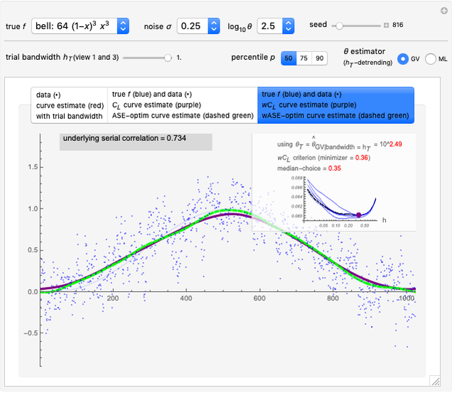
Here five examples for  (the "true curve") can be tried:
  is plotted (in blue) in the second and third of the three possible views using the tabs:
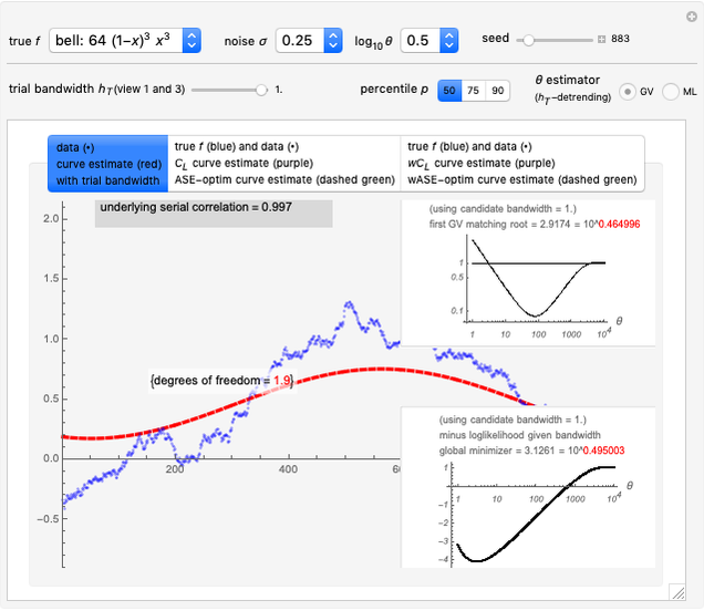
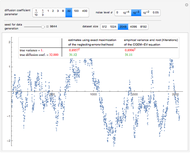
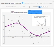
1. The first tab displays the data and the curve estimate  when
when  is set to a trial bandwidth
  ; the right-bottom panel displays a summary of the possible ML maximization when
  is subtracted, and the right-top panel displays the analog for GV matching.
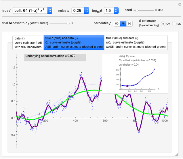
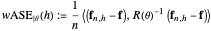
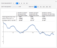
2. The second tab shows that the curve estimate (purple curve) produced by the non-modified  is very often quite undersmoothed. This tab also displays the ASE\[Hyphen]optimal choice (green curve), that is, the curve
  when
when  minimizes a global average of the squared errors between
  and
and  , defined by (where we denote by
  (resp.
  ) the
) the  column vector whose
  component is
  (resp.
  ), evaluated at
  )
)
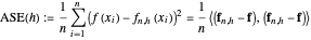 .
.
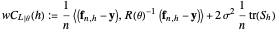
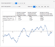
3. The third tab displays the results analog to tab 2, but this time we use a  -whitening, using either
  or
or  . Precisely, denoting by
  the correlation matrix of the underlying AR(1) time series when the inverse-range parameter is
  , that is, with
 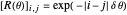 , the
, the  -whitened
  is
is
 .
.
Notice that when we denote by  the
the  column vector of observed data, whose
  component is thus
  , the
, the  -whitened
  is:
is:
 ,
,
where  is the smoothing matrix associated with the periodic kernel smoothing considered here. Since
  coincides with the
  identity matrix when
  , we are allowed to write in the legend of the panel in the second view that the results displayed here correspond to the choice
  .
.
In the first view, the underlying true function may be taken as the so-called bell-shaped polynomial, and the first tried bandwidth is the largest one (=1.): it can be observed that ML maximization and GV matching produce for each dataset (a new realization can be generated by changing the seed) two estimates of  that are very often near each other and that are good estimates of the true
  , and this is observed over a rather large range for
  . The observed fact that these estimates are not very impacted by the tried detrending is an appealing property of both ML and GV.
This third view assesses more precisely the impact of the goodness of these two estimates of  on the tuning of
  . In fact, it is demonstrated here that a property that is already well known for i.i.d. data still holds: the
  -whitened
  is often too flat near its minimum and always picking the exact minimizer is not the best tuning method when the ASE (or wASE) optimum is targeted. A simple solution we again propose here (as in the i.i.d. case) is to pick the upper quartile of the distribution of the randomized choices (more precisely using as in [6] the so-called augmented-randomization of the trace
  , see [7]): we can observe by varying the seed that this produces much more stable and often much better tuning of
  than always picking the median (quasi-equivalent to using the exact trace) when "better" means a lower ASE value on average.
References:
[1] C. Gu, Smoothing Spline Anova Models, 2nd ed., New York: Springer, 2013.
[2] D. A. Girard, "Estimating a Centered Ornstein–Uhlenbeck Process under Measurement Errors" from the Wolfram Demonstrations Project—A Wolfram Web Resource. demonstrations.wolfram.com/EstimatingACenteredOrnsteinUhlenbeckProcessUnderMeasurementE.
[3] D. A. Girard, "Estimating a Centered Matérn (1) Process: Three Alternatives to Maximum Likelihood via Conjugate Gradient Linear Solvers" from the Wolfram Demonstrations Project—A Wolfram Web Resource. demonstrations.wolfram.com/EstimatingACenteredMatern1ProcessThreeAlternativesToMaximumL.
[4] D. A. Girard, "Asymptotic Near-Efficiency of the 'Gibbs-Energy and Empirical-Variance' Estimating Functions for Fitting Matérn Models — I: Densely Sampled Processes," Statistics and Probability Letters, 110, 2016, pp. 191–197. doi:10.1016/j.spl.2015.12.021.
[5] D. A. Girard, "Efficiently Estimating Some Common Geostatistical Models by 'Energy–Variance Matching' or Its Randomized 'Conditional–Mean' Versions," Spatial Statistics, 21, 2017 pp. 1–26. doi:10.1016/j.spasta.2017.01.001.
[6] D. A. Girard, "Nonparametric Curve Estimation by Smoothing Splines: Unbiased-Risk-Estimate Selector and Its Robust Version via Randomized Choices," from the Wolfram Demonstrations Project—A Wolfram Web Resource. demonstrations.wolfram.com/NonparametricCurveEstimationBySmoothingSplinesUnbiasedRiskEs.
[7] D. A. Girard, "Estimating the Accuracy of (Local) Cross-Validation via Randomised GCV Choices in Kernel or Smoothing Spline Regression," Journal of Nonparametric Statistics, 22(1), 2010 pp. 41–64. doi:10.1080/10485250903095820.
Permanent Citation
 Estimating a Centered Ornstein-Uhlenbeck Process under Measurement Errors
Didier A. Girard Hierarchical Clustering and Heat Maps in Mathematica
Michael A Gibson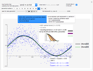 Nonparametric Regression and Kernel Smoothing: Confidence Regions for the L2-Optimal Curve Estimate
Didier A. Girard Kernel Density Estimation
Jeff Hamrick Dual Slope Analog-to-Digital Converter
Roy Rinberg PR4 Coding of a Magnetic Hard Drive
Charles Masenas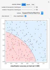 Comparison of Different Methods for the Binary Classification of Points in the Plane
Frank Brechtefeld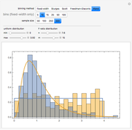 Automatically Selecting Histogram Bins
Brett Champion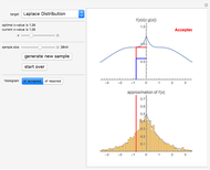 Acceptance/Rejection Sampling
Ryan Carroll and Jeff Hamrick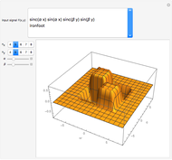 XFT2D: A 2D Fast Fourier Transform
Rafael G. Campos, J. Jesus Rico Melgoza, and Edgar Chavez
-
 Nonparametric Curve Estimation by Kernel Smoothers under Correlated Errors
Didier A. Girard -
 Estimators of a Noisy Centered Ornstein-Uhlenbeck Process and Its Noise Variance
Didier A. Girard -
 Nonparametric Density Estimation: Robust Cross-Validation Bandwidth Selection via Randomized Choices
Didier A. Girard -
 Nonparametric Additive Modeling by Smoothing Splines: Robust Unbiased-Risk-Estimate Selector and a Nonisotropic-Smoothing Improvement
Didier A. Girard -
 Nonparametric Curve Estimation by Smoothing Splines: Unbiased-Risk-Estimate Selector and its Robust Version via Randomized Choices
Didier A. Girard -
Estimating a Centered Ornstein-Uhlenbeck Process under Measurement Errors
Didier A. Girard -
 Estimating a Centered Matérn (1) Process: Three Alternatives to Maximum Likelihood via Conjugate Gradient Linear Solvers
Didier A. Girard -
 Three Alternatives to the Likelihood Maximization for Estimating a Centered Matérn (3/2) Process
Didier A. Girard -
Nonparametric Regression and Kernel Smoothing: Confidence Regions for the L2-Optimal Curve Estimate
Didier A. Girard -
 Nonparametric Curve Estimation by Kernel Smoothers: Efficiency of Unbiased Risk Estimate and GCV Selectors
Didier A. Girard