Pricing Put Options with the Crank-Nicolson Method


Requires a Wolfram Notebook System
Interact on desktop, mobile and cloud with the free Wolfram Player or other Wolfram Language products.
This Demonstration shows the application of the Crank–Nicolson (CN) method in options pricing. The CN method [1] is a central-time, central-space (CTCS) finite-difference method (FDM) for numerically solving partial differential equations (PDE). The CN scheme is the average of the implicit [2] and the explicit [3] schemes and can be used to numerically solve the Black–Scholes–Merton PDE [4, 5]. The CN scheme produces estimates of greater accuracy than either the explicit or implicit schemes.
Contributed by: Michail Bozoudis (December 2015)
Suggested by: Michail Boutsikas
Open content licensed under CC BY-NC-SA
Snapshots


Details
• The asset log price into  uniform steps with length
  , using
  nodes indexed
  .
.
• The option maturity time into  uniform steps with length
  , using
  nodes indexed
  .
.
Then  denotes the option value at the
  node. Three FDM schemas are widely used to approximate the derivatives:
• The Crank-Nicolson [1] scheme, also referred to as "central-time, central-space (CTCS)", uses the average of the above approximations. The error term of the CN scheme is  .
.
Compared to the implicit scheme, the explicit is considered simpler and faster but less stable and accurate. It is relatively accurate for a small number of steps. The explicit scheme is similar to the trinomial tree [6], in that both provide an explicit formula for determining future states of the option process in terms of the current state, whereas the implicit and CN schemas require the iterative solution of linear equations linking consecutive time steps.
You can use the controllers to select the put option parameters and to determine the log price and time steps of the spatial grid. The minimum and maximum limits of the log-price grid are automatically estimated in order to ensure convergence and stability. You can choose among three graphical displays:
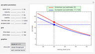
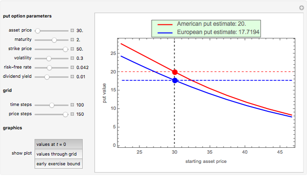
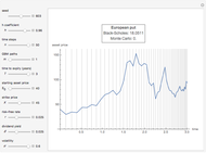
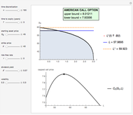
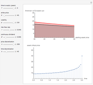
• The American and European put option estimates at  , depending on the underlying asset spot price. The European put value is never greater than the American, because the American put can be exercised at any time up to maturity, while the European put can only be exercised at maturity.
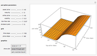
• The 3D illustration of the American put option values over the spatial grid.
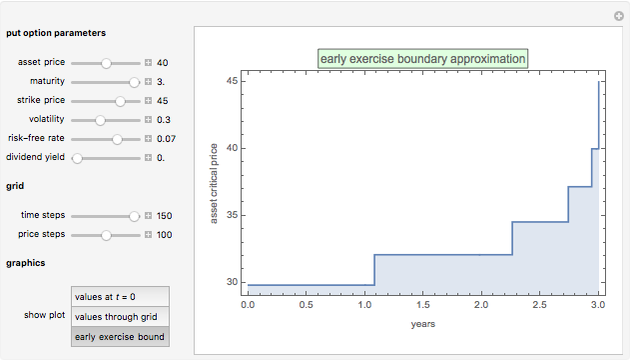
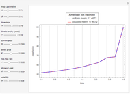
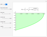
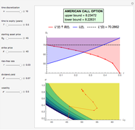
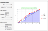
• The early exercise boundary approximation for the American put option. Whenever the asset price falls below this boundary, early exercise is considered optimal and the option is instantly exercised.
References
[1] J. Crank and P. Nicolson, "A Practical Method for Numerical Evaluation of Solutions of Partial Differential Equations of the Heat-Conduction Type," Proceedings of the Cambridge Philosophical Society, 43(1), 1947 pp. 50–67. doi:10.1017/S0305004100023197.
[2] M. J. Brennan and E. S. Schwartz, "Finite Difference Methods and Jump Processes Arising in the Pricing of Contingent Claims: A Synthesis," The Journal of Financial and Quantitative Analysis, 13(3), 1978 pp. 461–474. www.jstor.org/stable/2330152.
[3] J. Hull and A. White, "Valuing Derivative Securities Using the Explicit Finite Difference Method," Journal of Financial and Quantitative Analysis, 25(1), 1990 pp. 87–100. www.jstor.org/stable/2330889.
[4] F. Black and M. Scholes, "The Pricing of Options and Corporate Liabilities," Journal of Political Economy, 81(3), 1973 pp. 637–654. www.jstor.org/stable/1831029.
[5] R. Merton, "Theory of Rational Option Pricing," The Bell Journal of Economics and Management Science, 4(1), 1973 pp. 141–183. www.jstor.org/stable/3003143.
[6] P. Boyle, "Option Valuation Using a Three Jump Process," International Options Journal, 3(2), 1986 pp. 7–12.
Permanent Citation
 Pricing Put Options with the Trinomial Method
Michail Bozoudis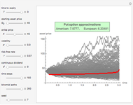 Pricing Put Options with the Binomial Method
Michail Bozoudis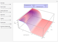 Pricing Put Options with the Explicit Finite-Difference Method
Michail Bozoudis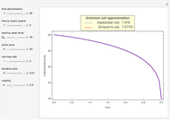 Kim's Method for Pricing American Options
Michail Bozoudis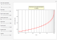 A Recursive Integration Method for Options Pricing
Michail Bozoudis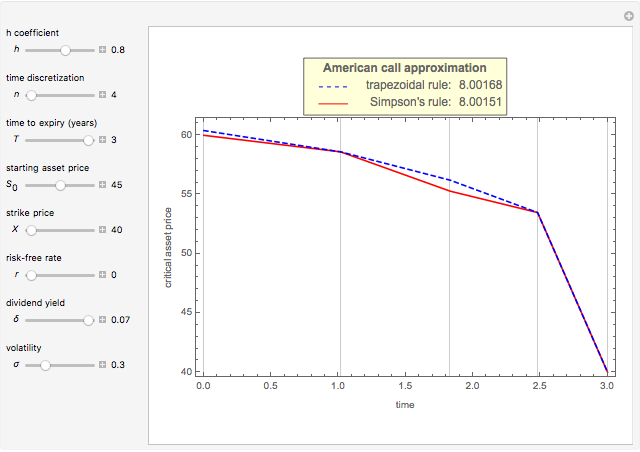 Kim's Method with Nonuniform Time Grid for Pricing American Options
Michail Bozoudis Adaptive Mesh Relocation-Refinement (AMrR) on Kim's Method for Options Pricing
Michail Bozoudis Pricing American Options with the Lower-Upper Bound Approximation (LUBA) Method
Michail Bozoudis Pricing American Options with the Two- and Three-Point Maximum Methods
Michail Bozoudis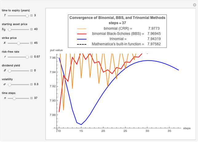 Convergence of Binomial, Binomial Black-Scholes, and Trinomial Option Pricing Methods
Michail Bozoudis
-
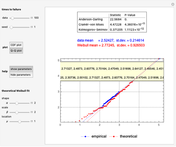 Fitting Times-to-Failure to a Weibull Distribution
Michail Bozoudis -
 A Canonical Optimal Stopping Problem for American Options
Michail Bozoudis -
A Recursive Integration Method for Options Pricing
Michail Bozoudis -
Adaptive Mesh Relocation-Refinement (AMrR) on Kim's Method for Options Pricing
Michail Bozoudis -
Kim's Method with Nonuniform Time Grid for Pricing American Options
Michail Bozoudis -
 Geometric Brownian Motion with Nonuniform Time Grid
Michail Bozoudis -
Kim's Method for Pricing American Options
Michail Bozoudis -
 Simultaneous Confidence Interval for the Weibull Parameters
Michail Bozoudis -
 Binomial Black-Scholes with Richardson Extrapolation (BBSR) Method
Michail Bozoudis -
Pricing American Options with the Lower-Upper Bound Approximation (LUBA) Method
Michail Bozoudis -
 American Options on Assets with Dividends Near Expiry
Michail Bozoudis -
 Hold-or-Exercise for an American Put Option
Michail Bozoudis -
 American Capped Call Options with Exponential Cap
Michail Bozoudis -
 American Capped Call Options with Constant Cap
Michail Bozoudis -
 Pricing Put Options with the Crank-Nicolson Method
Michail Bozoudis -
 Pricing Put Options with the Implicit Finite-Difference Method
Michail Bozoudis -
 Estimating a Distribution Function Subject to a Stochastic Order Restriction
Michail Bozoudis -
 Maximizing a Bermudan Put with a Single Early-Exercise Temporal Point
Michail Bozoudis -
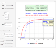 Fitting Data to a Lognormal Distribution
Michail Bozoudis -
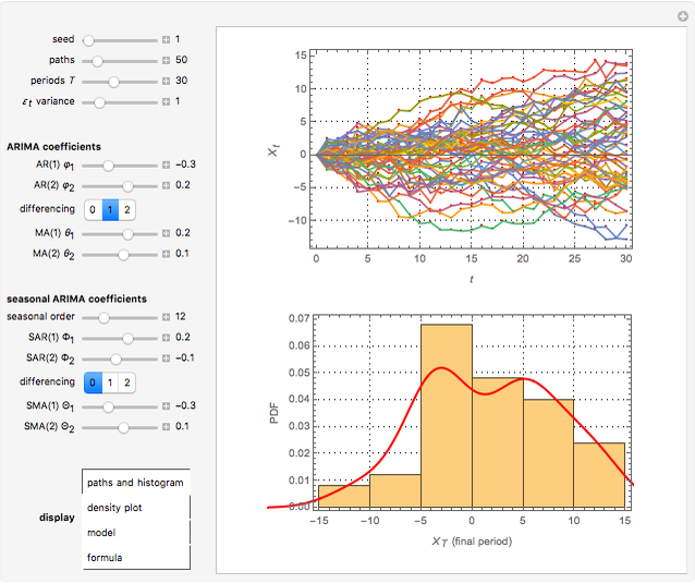 SARIMA Process Forecasting Model
Michail Bozoudis