Quantum Random Walk


Requires a Wolfram Notebook System
Interact on desktop, mobile and cloud with the free Wolfram Player or other Wolfram Language products.
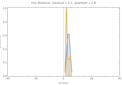
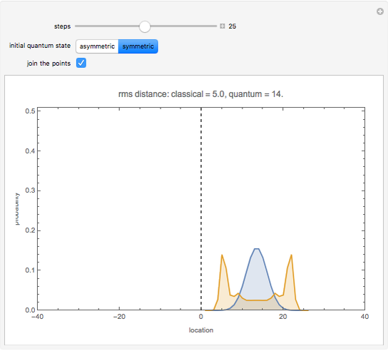
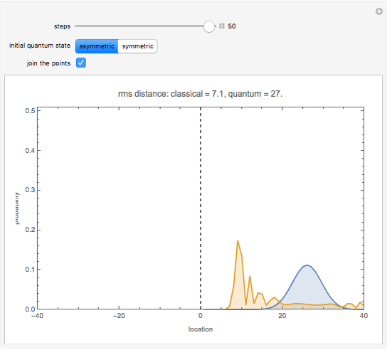
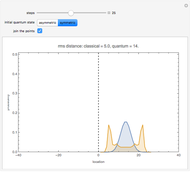
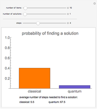
This Demonstration shows the probability distribution for discrete classical and quantum random walks on a line, starting from the location marked 0. The controls vary the number of steps for the walk and, for the quantum case, whether the initial state is symmetric or not. The plot label gives the root mean square (rms) distance of the walk from the origin after the specified number of steps.
Contributed by: Tad Hogg (March 2011)
Open content licensed under CC BY-NC-SA
Snapshots


Details
Snapshot 1: with the symmetric initial state, the probability for the quantum walk is symmetric about the origin
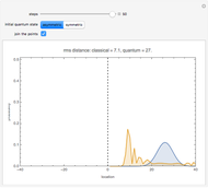
Snapshot 2: after many steps, the particle performing a quantum random walk is likely to be much farther from the origin than with a classical random walk
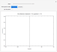
Snapshot 3: after just one step, both classical and quantum random walks have the same probabilities: equally likely to be at positions +1 or -1
In the classical random walk, at each step there is equal probability for the particle to move one unit to the left or right along the line. During a single random walk, the particle is at a definite location after each step. The probability shown in the plot is the fraction of such walks in which the particle is at each location after the specified number of steps.
In the quantum random walk, the particle is in a superposition of locations along the line. The values shown in the plot are the probability of finding the particle at each location if the particle is observed after the specified number of steps.
The state of the quantum particle after  steps can be expressed as a sum
  , where the
  values are complex numbers,
  is an integer between
  and giving the location along the line, and
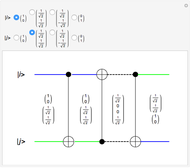
  is a single quantum bit (called a qubit) that represents the value of a coin flipped to determine the direction of the particle at the next step: 0 and 1 correspond to decreasing and increasing by 1, respectively. The probability of observing the particle at location is
  .
.
After a step, the superposition becomes 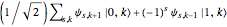 . Thus a quantum particle starting at a definite location
  has equal probability of being observed after one step at locations
  or
or  , the same as the classical random walk. But after more than one step, interference among multiple terms in the superposition gives different behavior between the classical and quantum random walks.
The behavior of the quantum random walk varies with the choice of initial state for the qubit  . This qubit can start with a definite state (0 or 1), the same as a classical bit. More generally, the qubit can start as a superposition of the two values 0 and 1. This Demonstration shows two examples for the initial state of the qubit. The asymmetric initial condition has
  and all other values equal to zero. The symmetric initial condition has
  ,
,  , and all other values equal to zero. In both cases, the particle starts at location 0, the same as for the classical random walk.
After an even or odd number of steps, the particle can only be at even or odd locations along the line, respectively. Selecting the "join the points" control shows a curve connecting the nonzero probabilities.
For further details and generalizations, see J. Kempe, "Quantum Random Walks: An Introductory Overview," Contemporary Physics, 44, 2003 pp. 307–327.
For a physical implementation, see M. Karski et al., "Quantum Walk in Position Space with Single Optically Trapped Atoms," Science, 325, 2009 pp. 174–177.
Permanent Citation
 Swapping Qubit States
Brad Rubin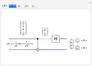 Measuring Entangled Qubits
Brad Rubin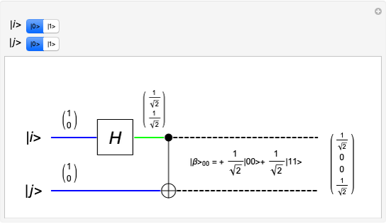 Generating Entangled Qubits
Brad Rubin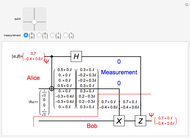 Quantum Teleportation
Brad Rubin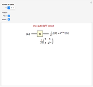 Quantum Fourier Transform Circuit
Rudolf Muradian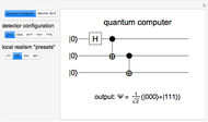 Quantum Computer Simulation of GHZ Experiment
S. M. Blinder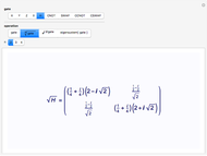 Quantum Logic Gates: Roots, Exponents, and Eigensystems
Rudolf Muradian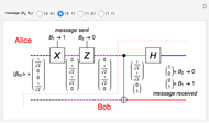 Superdense Coding
Brad Rubin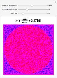 Approximating Pi by the Monte Carlo Method
Zubeyir Cinkir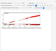 Simulating a Multiple Server Queue
Karl W. Heiner (SUNY New Paltz) and Stan Wagon (Macalester College)
-
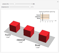 Compressing Ideal Fermi and Bose Gases at Low Temperatures
Tad Hogg -
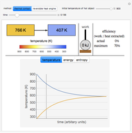 Irreversible and Reversible Temperature Equilibration
Tad Hogg -
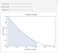 Maximum Likelihood Estimation for Coin Tosses
Tad Hogg -
 Stroop Effect: Reading Colored Words
Tad Hogg -
 Bijective Mapping of an Interval to a Square
Tad Hogg -
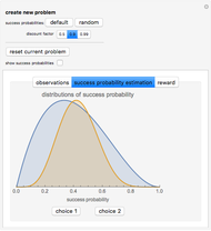 The Multi-Arm Bandit
Tad Hogg -
 Juggling the Cascade Pattern
Tad Hogg -
 Quantum Random Walk
Tad Hogg -
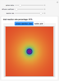 Diffusion to a Spherical Reactor
Tad Hogg -
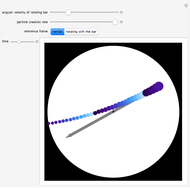 Particles Thrown from a Rotating Bar
Tad Hogg -
 Grover's Quantum Search Algorithm
Tad Hogg -
 Simulated Quantum Computer Algorithm for Database Searching
Tad Hogg -
 Quantum Computer Search Algorithms
Tad Hogg