Simulating the Bernoulli-Laplace Model of Diffusion

Requires a Wolfram Notebook System
Interact on desktop, mobile and cloud with the free Wolfram Player or other Wolfram Language products.
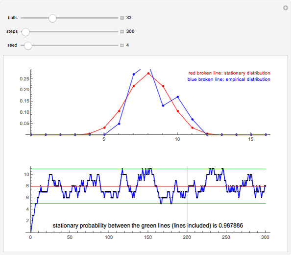
This Demonstration simulates a special discrete-time Markov chain, the so-called Bernoulli–Laplace model of diffusion. In this model, there are two urns; initially, urn I contains exactly  black balls and urn II contains exactly
  white balls. Repeat the following experiment: one ball is selected at random from each of the urns. The ball selected from urn I is put into urn II and the ball selected from urn II is put into urn I. During such a sequence of experiments, we consider the number of white balls in urn I. The resulting random process is a discrete-time Markov chain.
Contributed by: Heikki Ruskeepää (March 2011)
Open content licensed under CC BY-NC-SA
Snapshots
Details
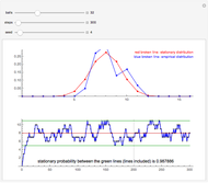
Snapshot 1: 300 steps from which the last 100 steps are used to estimate the state probabilities; the estimated probabilities are quite poor
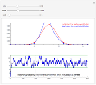
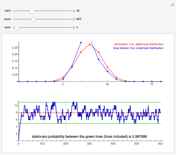
Snapshot 2: 600 steps from which the last 400 steps are used to estimate the state probabilities; the estimated probabilities are better but still differ considerably from the stationary distribution
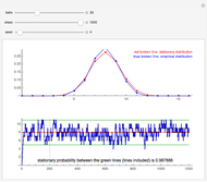
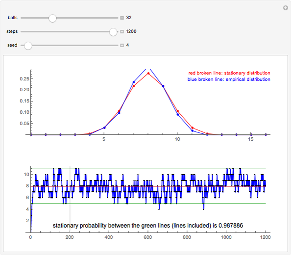
Snapshot 3: 1200 steps from which the last 1000 steps are used to estimate the state probabilities; the estimated probabilities are quite close to the stationary distribution
For example, suppose there are 32 balls, 16 of which are white and 16 black. At the start of the simulation, urn I contains 0 white balls and 16 black balls. The number of white balls in urn I grows so that it has, in the long run, approximately 8 white balls and 8 black balls. From the snapshots, the probability that the state (the number of white balls in urn I) is between the green lines is 0.988 in a stationary situation, that is, the state is among 5, 6, 7, 8, 9, 10, and 11 with this probability. The green lines are calculated so that they give at least 95% confidence intervals (the given probability is exact).
We calculate the stationary probabilities from the well-known linear equations. However, the example considered allows a closed-form solution for the equations, see, [1, p. 398]. We use the equations to enable the user of the Demonstration to also easily simulate other discrete-time Markov chains.
When the empirical distribution is calculated, we reject the first 200 steps as transient.
For the Bernoulli-Laplace model of diffusion, see [1]. For simulation of the discrete-time Markov chain and other stochastic processes with Mathematica, see [2].
[1] W. Feller, An Introduction to Probability Theory and Its Applications, Vol. I, 3rd ed., revised printing, pp. 378, 397, New York: Wiley.
[2] H. Ruskeepää, Mathematica Navigator: Mathematics, Statistics, and Graphics, 3rd ed., pp. 987–1002, San Diego, CA: Elsevier Academic Press, 2009.
Permanent Citation
"Simulating the Bernoulli-Laplace Model of Diffusion"
http://demonstrations.wolfram.com/SimulatingTheBernoulliLaplaceModelOfDiffusion/
Wolfram Demonstrations Project
Published: March 7 2011


