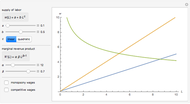
Supply Curve from Piecewise Linear Cost Function


Requires a Wolfram Notebook System
Interact on desktop, mobile and cloud with the free Wolfram Player or other Wolfram Language products.
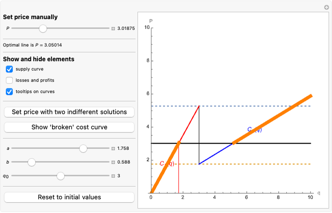
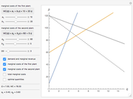
This Demonstration shows how to define a supply curve if a marginal cost curve is piecewise and "broken." The problem of the price-taking competitive firm is to define which quantity to produce if the price is set in the range between two edge points, or, to put it differently, which piece of the cost curve to use to define the quantity  given the price,
  , where
  is given. For simplicity, we consider linear cost functions (and that the average cost curve intersects the marginal cost curve at the origin). We show the principal approach to the problem, which can be generalized to arbitrary cost functions with many break points.
Contributed by: Timur Gareev (October 2015)
Immanuel Kant Baltic Federal University
Open content licensed under CC BY-NC-SA
Details
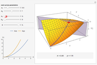
Suppose we know that a firm has a piecewise cost function of the following form:  if
if  and
and  if
if  , where
  and where
  is constant and stands for a given quantity where the cost curve breaks between the
  and
and  pieces (we may change it with the respective control). This outset differs from the usual case with
  in the following point: the firm should define what quantity
  to produce if the market price is in the range
  (i.e. it has two options: to use
  or
or  pieces). In more general terms, the firm should define its supply curve, which does not simply coincide with the cost curve in this case. Note that if the firm produces according to the first piece of the cost curve,
  , there is nothing special to analyze. But if the firm switches to the
  piece of the cost curve, then there is a challenge: is it profitable or not? Indeed, to move to the
  piece, given the price, there are first some losses before the "breaking" quantity
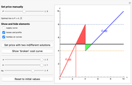
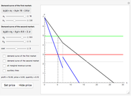
  level of production, and then some profits. (See this by changing the
  slider and observing the red and green triangles.) The trick is to integrate those triangles to define the break-even price level
  , where the producer is indifferent between two pieces of the cost curve. This price
  is found by solving the following equation:
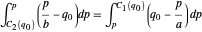 .
.
This price level allows us to define the horizontal "break" level of the supply curve (can be shown by the checkbox on the graph). This also means that the red and green triangles on the graph have equal areas. In economic terms, red corresponds to losses and green reflects profits. When profits and losses are equal, the producer is indifferent between the two alternatives, so the supply curve (derived from the marginal cost curve lying above the average cost curve) has a discontinuity between the two indifferent solutions. In this "problematic" range of prices  , one cannot switch to the
  piece of the cost curve without suffering some losses that should be compensated by additional profits. (You can see the supply curve on the graph by checking the checkbox of the respective control.) As a result, we may define the supply curve that becomes discontinuous in this model.
Snapshots


Permanent Citation
 Revenue and Costs Curves Analysis
Timur Gareev Elasticity Function
Timur Gareev Firm Costs Optimization Problem in Primal and Dual Form
Timur Gareev Returns to Scale in One-Factor Production Functions
Timur Gareev Isocosts, Isoquants, Isocline Lines, and Scale Lines for Homogeneous (Cobb-Douglas) Functions
Timur Gareev Short-Run Cost Curves
William J. Polley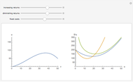 Short-Run Production and Cost Curves
Tom Creahan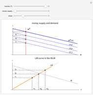 Deriving the Liquidity Preference-Money Supply (LM) Curve
Nicholas Palmer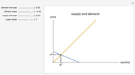 Basic Supply and Demand
Mark Gillis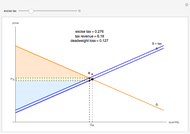 Supply and Demand Excise Tax
Nicholas Palmer
-
 Supply Curve from Piecewise Linear Cost Function
Timur Gareev -
 Krugman's Model of Increasing Returns and Monopolistic Competition
Timur Gareev -
Returns to Scale in One-Factor Production Functions
Timur Gareev -
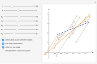
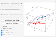 Omitted Variable Bias in 3D
Timur Gareev -
Revenue and Costs Curves Analysis
Timur Gareev -
 Leontief Production Function
Timur Gareev -
 Simultaneity Bias
Timur Gareev -
Firm Costs Optimization Problem in Primal and Dual Form
Timur Gareev -
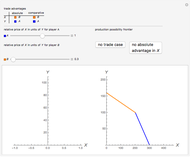 Comparative and Absolute Advantage
Timur Gareev -
 Firm with Two Plants
Timur Gareev -
Elasticity Function
Timur Gareev -
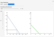 Substitute and Complementary Goods
Timur Gareev -
 Monopoly with Two Plants
Timur Gareev -
 Best Response in Static Two-Player Games
Timur Gareev -
 Hotelling Model of Product Quality Differentiation
Timur Gareev -
 Endogeneity Bias
Timur Gareev -
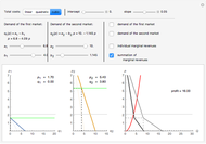 Discriminating Monopolist with Two Independent Markets
Timur Gareev -
 Monopsony in the Labor Market
Timur Gareev -
 Nondiscriminating Monopolist with Two Independent Markets
Timur Gareev -
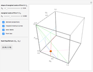 Duopoly Model in 3D
Timur Gareev