The Basic Keynesian Expenditure Model


Requires a Wolfram Notebook System
Interact on desktop, mobile and cloud with the free Wolfram Player or other Wolfram Language products.
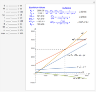
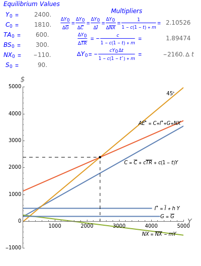
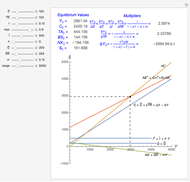
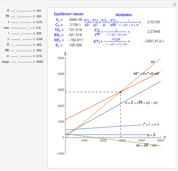
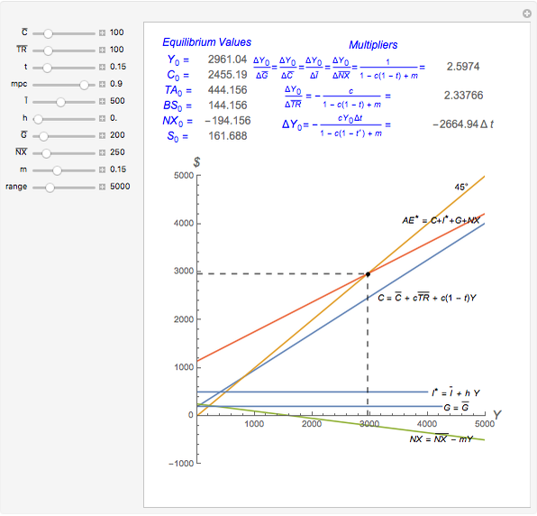
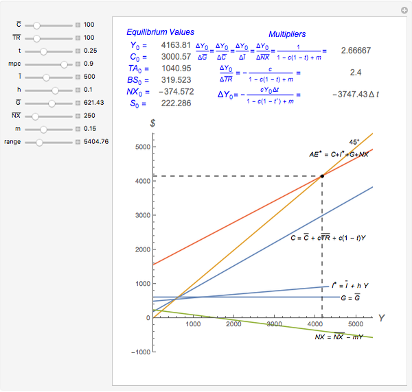
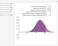
This Demonstration presents a simple Keynesian macroeconomic expenditure model without financial assets or exchange rates. The table provides equilibrium values of real GDP, personal consumption expenditures, tax revenue, budget surplus, trade surplus, and personal savings. The table shows autonomous spending multipliers (i.e. government spending, autonomous consumption, autonomous investment, and autonomous net exports) as well as the income tax rate multiplier.
Contributed by: Craig S. Marcott (July 2011)
Open content licensed under CC BY-NC-SA
Snapshots


Details
The notation is fairly standard in macroeconomics, but most closely follows the Dornbusch, Fischer, and Startz text [1].
 = real GDP (i.e. market value of all final goods and services produced in a country during a year)
 = tax revenue
 = government transfer payments (i.e. payments people receive as income from the government, but for which no productive service has been rendered in the current time period)
 = disposable income
 = personal consumption expenditures (i.e. durables + nondurables + services)
 = gross private domestic investment (i.e. new residential construction + new plant and equipment + change in inventories)
 = personal savings ≡
 = government purchases of goods and services
 = net exports (i.e. exports – imports); this is also called the trade surplus
 = budget surplus
 ≡ desired investment (i.e. new residential construction + new plant and equipment + desired inventory change)
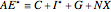 = desired aggregate expenditure
 (national income accounting identity)
Autonomous spending is a constant value of spending that is taken as given (i.e. determined outside of the model). Autonomous values are denoted with an overbar (i.e.  ,
,  ,
,  ,
,  ,
,  ).
).
Keynesian equilibrium condition:  . The intuition behind this condition is that the firms of the economy adjust their production levels to bring into line actual and desired inventory changes. For example, if
  , then
  and
and  . From the definitions of actual and desired investment, this means the desired inventory change exceeds the actual inventory change. There is unintended inventory depletion and firms respond by increasing production (i.e. to replenish inventories). This causes to increase until . A similar argument can be used to show that real GDP will fall whenever
  . (That is,
  desired inventory change
  actual inventory change
  unintended inventory accumulation firms produce less falls.)
Equilibrium values are denoted with a zero subscript (i.e.  ,
,  ,
,  ,
,  ,
,  ,
,  ). These are obtained by substituting the equilibrium value of real GDP () into the corresponding behavioral equation.
Equations specifying the behavior of the macroeconomic aggregates
(1)  ;
; 
The parameter  is the marginal propensity to consume (i.e. the additional consumption spending associated with an additional dollar of disposable income).
(2)  ;
; 
The parameter  is the marginal propensity to invest (i.e. the additional desired investment spending associated with an additional dollar of real GDP).
(3) 
(4)  ;
; 
The parameter  is the marginal propensity to import (i.e. the additional import spending associated with an additional dollar of real GDP).
(5)  ;
; 
The parameter  is the marginal tax rate or the marginal propensity to tax (i.e. the additional tax revenue associated with an additional dollar of real GDP).
The multipliers give the rate of change of equilibrium real GDP
 ≡ government spending multiplier (i.e. the change in equilibrium real GDP associated with a one dollar change in )
 ≡ autonomous investment multiplier (i.e. the change in equilibrium real GDP associated with a one dollar change in autonomous investment)
 ≡ autonomous consumption multiplier (i.e. the change in equilibrium real GDP associated with a one dollar change in autonomous consumption)
 ≡ transfer payment multiplier (i.e. the change in equilibrium real GDP associated with a one dollar change in autonomous transfer payments)
 ≡ autonomous net export multiplier (i.e. the change in equilibrium real GDP associated with a one dollar change in autonomous net export spending)
Since the impact of a change in the marginal tax rate depends on the initial equilibrium value of real GDP, this "multiplier" is not stated as a ratio. In this model the change in equilibrium output is
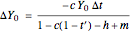 , where
  is the new tax rate.
Reference
[1] R. Dornbusch, S. Fischer, and R. Startz, Macroeconomics, 11th ed., New York: McGraw–Hill, 2011.
Permanent Citation
 Capacity Planning for Short Life Cycle Products: The Newsvendor Model
Shailesh S. Kulkarni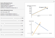 The Keynesian IS-LM Model
William J. Polley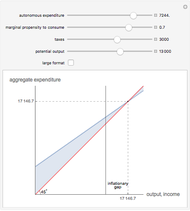 Keynesian Cross Diagram
Fiona Maclachlan Basic Option Trading Strategies
Peter Falloon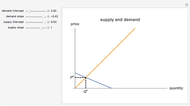 Basic Supply and Demand
Mark Gillis Monopoly Model
David Youngberg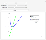 Competitive Model
David Youngberg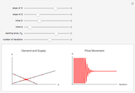 Cobweb Model
Samuel G. Chen Simple Solow Model
Alex Tabarrok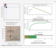 Bilateral Accident Model
Seth J. Chandler