The Three-Dimensional Isotonic Potential in Bohmian Mechanics

Requires a Wolfram Notebook System
Interact on desktop, mobile and cloud with the free Wolfram Player or other Wolfram Language products.
In quantum chemistry the study of exact solutions of the Schrödinger equation for an harmonic oscillator with a centripetal barrier, called the three-dimensional isotonic oscillator or pseudoharmonic potential, is of considerable interest. Diatomic molecules contain two atoms that are chemically bonded; homonuclear if the two atoms are identical, such as the oxygen molecule  , heteronuclear if the atoms are different, as carbon monoxide
  . The three-dimensional version in spherical polar coordinates of the isotonic potential for a heteronuclear diatomic molecule in the de Broglie–Bohm approach (often called Bohmian mechanics or causal interpretation of quantum mechanics) is considered here.


Contributed by: Klaus von Bloh (May 2021)
Open content licensed under CC BY-NC-SA
Snapshots


Details
The three-dimensional stationary Schrödinger equation with potential  and with the reduced mass
  can be written as
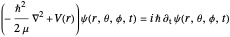 ,
,
with the Laplacian  in spherical polar coordinates and the partial derivative
  with respect to time.
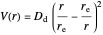
With the three-dimensional isotonic or pseudoharmonic potential [3–5]:
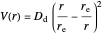 .
.
The eigenfunctions can be expressed in spherical coordinates in a separable form:
 .
.
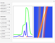
The unnormalized radial  wavefunction is expressed in terms of the associated Laguerre polynomials
  and the angular part is expressed in terms of spherical harmonics
  .
.
The radial term is:
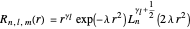
with
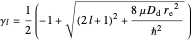
and

as the radial part.
The explicit bound state energies are obtained from (for more details see [5]):
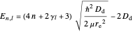 .
.
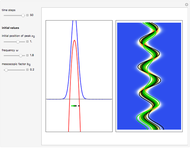
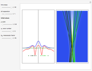
To use the time dependence of the total phase function, the superposed wavefunctions Ψ are taken as a sum of just two eigenfunctions  , where the unnormalized wavefunction
  for a particle is written as:
 ,
,
with  and integers
  ,
,  and
and  and, here, with
  and
and  ,
,  ,
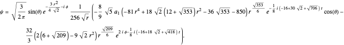
,  and with the remaining term in atomic units. In spherical polar coordinates, the total wavefunction becomes:
After a variable transformation from spherical polar coordinates into Cartesian coordinates, one obtain the phase function  . From the gradient of the phase
  from the total wavefunction
  in the eikonal (or polar) form
  , with the quantum amplitude
  , the velocity field
  is calculated using:
 .
.
For  or
or  , the velocity field
  becomes autonomous and obeys the time-independent part of the continuity equation
  with
with  ; for
; for  or
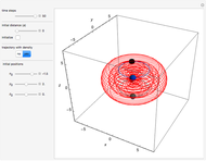
or  the trajectories reduce to circles with the velocities
  and
and  , but with different signs:
and
 ,
,
where the velocity depends only on the position of the particle.
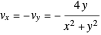
For the special initial positions ( ,
,  and
and  ) and with time
  , the velocity vector becomes autonomous in the
  and
and  directions, but not in the
  direction:
 ;
;
and
For  , please refer to the code.
In this special case it is interesting to find initial positions where the  component of the velocity becomes negligibly small. This could be achieved for some values of the intersection of the equation
 ;
;
for example,
 ,
,
and  or for the trial solution with
  ,
,  ,
,  .
.
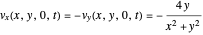
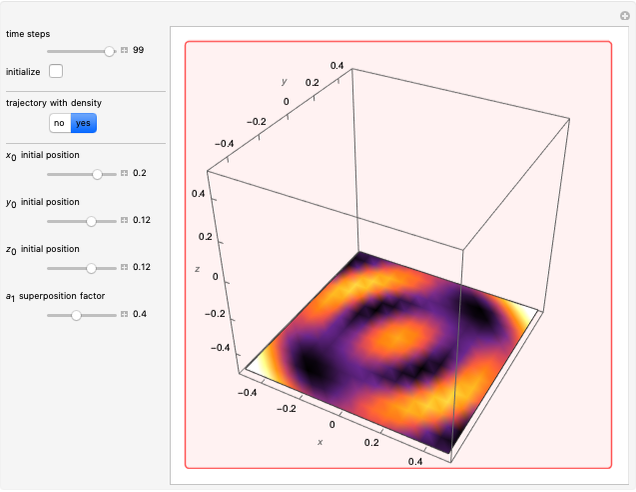
In the very special cases the velocities vector in the  and
and  directions become autonomous (
 ) and
) and  becomes negligibly small (
 ) for all times
  . These orbits do not leave the
  plane.
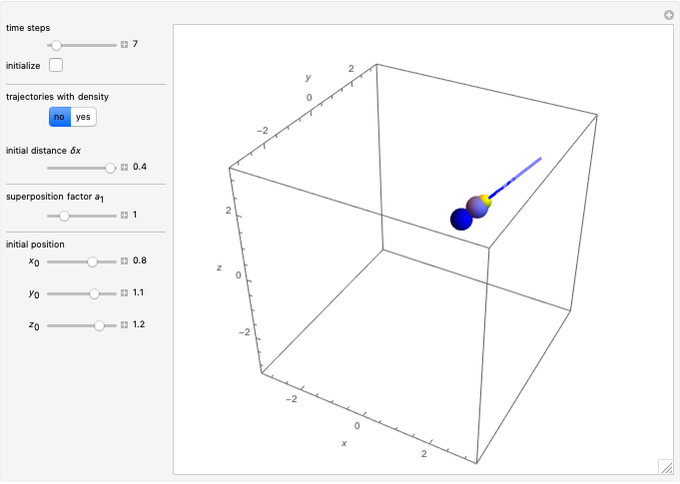
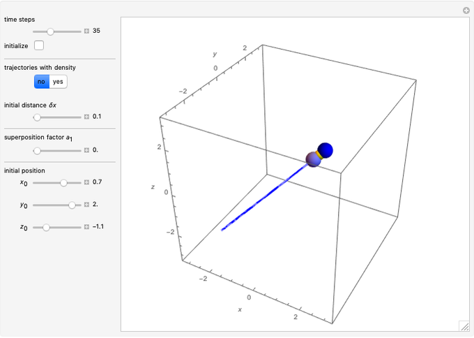
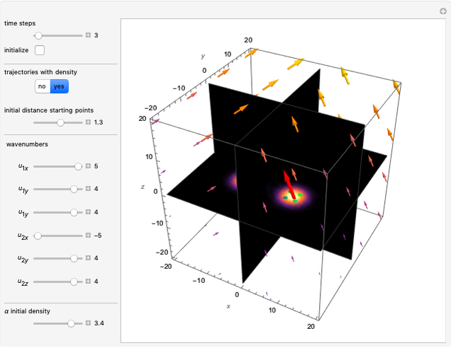
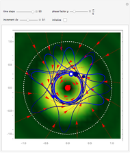
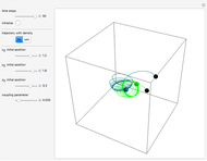
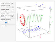
In all other cases, the velocity vector  becomes very complicated and the orbits appear to be unstable or ergodic. This means that as the trajectory evolves in time, the entire possible configuration space will be occupied by the orbit, that is, the orbits are dense everywhere. For some initial positions, the orbit will be closed and periodic (regular). It is not obvious for this system with two superposed eigenfunctions that chaotic motion occurs, which would be associated with exponential divergence of initially neighboring trajectories [6–8]. Further investigations are needed to get the full dynamics of the system.
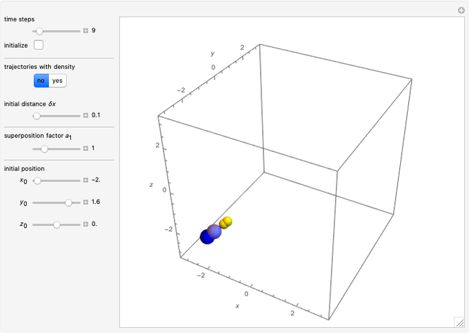
When PlotPoints, AccuracyGoal, PrecisionGoal and MaxSteps are increased (if enabled), the results will be more accurate. The initial distance between the two starting trajectories is determined by the factor  .
.
The author would like to thank Ilka Weiß for helpful discussions.
References
[1] Bohmian-Mechanics.net. (Apr 8, 2021) bohmian-mechanics.net.
[2] S. Goldstein, "Bohmian Mechanics." The Stanford Encyclopedia of Philosophy (Summer 2017 Edition). (Apr 8, 2021) plato.stanford.edu/entries/qm-bohm.
[3] P. M. Davidson, "Eigenfunctions for Calculating Electronic Vibrational Intensities," Proceedings of the Royal Society A, 135(827), 1932 pp. 459–472. doi:10.1098/rspa.1932.0045.
[4] Y. Weissman and J. Jortner, "The Isotonic Oscillator," Physics Letters A, 70(3), 1979 pp. 177–179. doi:10.1016/0375-9601(79)90197-X.
[5] K. J. Oyewumi and K. D. Sen, "Exact Solutions of the Schrödinger Equation for the Pseudoharmonic Potential: An Application to Some Diatomic Molecules," Journal of Mathematical Chemistry, 50(5), 2012 pp. 1039–1059. doi:10.1007/s10910-011-9967-4.
[6] R. H. Parmenter and R. W. Valentine, "Deterministic Chaos and the Causal Interpretation of Quantum Mechanics," Physics Letters A, 201(1), 1995 pp. 1–8. doi:10.1016/0375-9601(95)00190-E.
[7] A. C. Tzemos, G. Contopoulos and C. Efthymiopoulos,"Origin of Chaos in 3-D Bohmian Trajectories," Physics Letters A, 380(45), 2016 pp. 3796–3802. doi:10.1016/j.physleta.2016.09.016.
[8] K. von Bloh. The Three-Dimensional Isotonic Potential in the Bohmian Mechanics Approach. [Video]. (Apr 8, 2021) www.youtube.com/watch?v=gZz7jsosG6Y.
Permanent Citation
 Ontology of the One-Dimensional Wavefunction in Bohmian Mechanics
Klaus von Bloh Nodal Points in Bohmian Mechanics
Klaus von Bloh Bohm Trajectories for the Two-Dimensional Coulomb Potential
Klaus von Bloh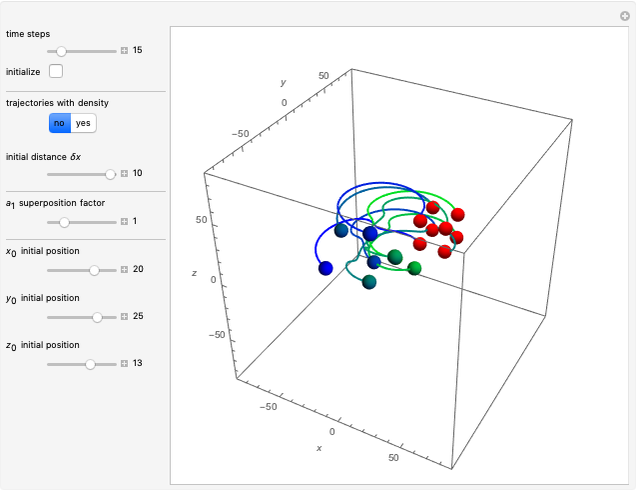 Bohm Trajectories for the Noncentral Hartmann Potential
Klaus von Bloh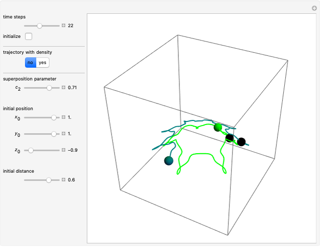 Quantum Orbits of a Particle in Spherical Coordinates in a Three-Dimensional Harmonic Oscillator Potential
Klaus von Bloh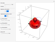 The sp Hybrid Orbital in Bohmian Mechanics
Klaus von Bloh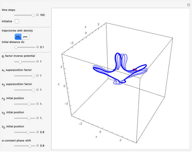 Bohm Trajectories for a Special Type of a Pseudoharmonic Potential
Klaus von Bloh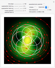 Bohm Trajectories for an Isotropic Harmonic Oscillator with Added Inverse Quadratic Potential
Klaus von Bloh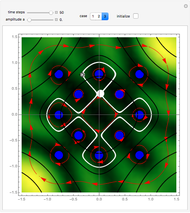 Bohmian Quantum Trajectories for Coherent States of the Pöschl-Teller Potential
Klaus von Bloh Bohm Trajectories for a Particle in a Two-Dimensional Calogero-Moser Potential
Klaus von Bloh
-
 The Three-Dimensional Isotonic Potential in Bohmian Mechanics
Klaus von Bloh -
Ontology of the One-Dimensional Wavefunction in Bohmian Mechanics
Klaus von Bloh -
Bohm Trajectories for the Noncentral Hartmann Potential
Klaus von Bloh -
Bohm Trajectories for a Special Type of a Pseudoharmonic Potential
Klaus von Bloh -
 Collision of Two Neutrons in the de Broglie?Bohm Approach
Klaus von Bloh -
 Quantum Motion in an Infinite Spherical Well
Klaus von Bloh -
The sp Hybrid Orbital in Bohmian Mechanics
Klaus von Bloh -
Quantum Orbits of a Particle in Spherical Coordinates in a Three-Dimensional Harmonic Oscillator Potential
Klaus von Bloh -
Bohm Trajectories for an Isotropic Harmonic Oscillator with Added Inverse Quadratic Potential
Klaus von Bloh -
Bohm Trajectories for the Two-Dimensional Coulomb Potential
Klaus von Bloh -
 Bohm Trajectories in an LCAO Approximation for the Hydrogen Molecule H_2
Klaus von Bloh -
 Decoherence and Trajectories Implied by a Modified Schrodinger Equation
Klaus von Bloh -
 Bohm Trajectories for a Particle in a Two-Dimensional Circular Billiard
Klaus von Bloh -
 From Bohm to Classical Trajectories in a Hydrogen Atom
Klaus von Bloh -
 Continuous Transition between Quantum and Classical Behavior for a Harmonic Oscillator
Klaus von Bloh -
 Continuous Transition between Classical and Bohm Quantum Pictures for Young's Interference Experiment
Klaus von Bloh -
 Bohm Trajectories for Quantum Particles in a Uniform Gravitational Field
Klaus von Bloh -
Bohm Trajectories for a Particle in a Two-Dimensional Calogero-Moser Potential
Klaus von Bloh -
 Nonlocality in the de Broglie-Bohm Interpretation of Quantum Mechanics
Klaus von Bloh -
 Three-Soliton Collision in the Trajectory Approach
Klaus von Bloh