Two-Phase Simplex Method

Requires a Wolfram Notebook System
Interact on desktop, mobile and cloud with the free Wolfram Player or other Wolfram Language products.
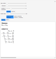
This Demonstration computes the solution of a randomly generated linear programming problem using the two-phase simplex algorithm. It displays the table generated while stepping through the simplex algorithm and then compares the solution so obtained with Mathematica's built-in function LinearProgramming.
Contributed by: Sourav Mukherjee (June 2011)
Open content licensed under CC BY-NC-SA
Snapshots


Details
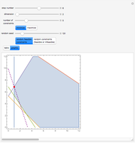
Phase 1 of the two-phase simplex algorithm tries to find a basic feasible solution. Artificial variables  are introduced in phase 1 and dropped at the beginning of phase 2. If the constraints are feasible, then the basic feasible solution obtained at the end of phase 1 is used in phase 2 to begin a search for the optimal solution (which lies at one of the corners of the convex polytope defined by the constraint equations). The
  denote slack variables.
In phase 1, the top row of the table represents the objective equation  that we try to minimize to zero in our search for a basic feasible solution. The second row from the top represents our actual objective function
  in phase 1.
At the beginning of phase 2, the top row is dropped and the new top row represents the actual objective function .
If the linear programming problem immediately offers a basic feasible solution, phase 1 is bypassed. No artificial variables are introduced.
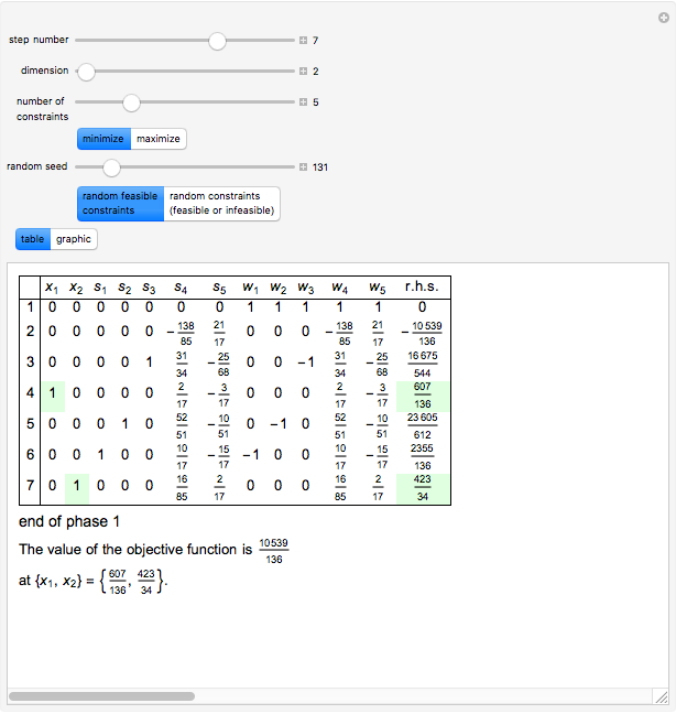
If the value in the right-hand side (r.h.s.) column of the top row is negative at the end of phase 1, it means that the constraints are infeasible.
An equality constraint is replaced by the corresponding greater-than-equal-to constraint and the lesser-than-equal-to constraint.
In this Demonstration, in the tables the values attained by the original variables that happen to be basic variables are highlighted in light green. The pivot element is highlighted in light red. The value attained by the objective function at the end of phase 2 is highlighted in light blue.
In two-dimensional cases, the value attained by the original variables  as inferred from the table is indicated by a red dot in the corresponding graphic.
For details of the algorithm used, please refer to Chapter 3 of [1].
Reference
[1] S. S. Rao, Engineering Optimization:Theory and Practice, 3rd ed., New Delhi: New Age International, 2006.
Permanent Citation
 Affine-Scaling Interior Point Method
Andreas Lauschke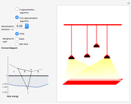 Stage Illumination Problem
Slobodan Jelic and Domagoj Matijevic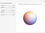 Shortest Path between Two Points on a Sphere
Bernard Vuilleumier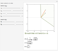 Farkas's Lemma in Two Dimensions
Tetsuya Saito 0-1 Knapsack Problem
Conrad A. Benulis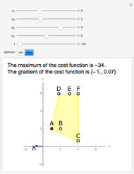 Parametric Linear Programming
Bunduchi Ecaterina and Mandric Igor Frobenius Equation in Two Variables
Izidor Hafner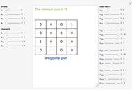 Monge-Kantorovich Transportation Problem
Mandric Igor (Moldova State University) Computable General Equilibrium (CGE) of Multiregion Input-Output Model
Stuart Nettleton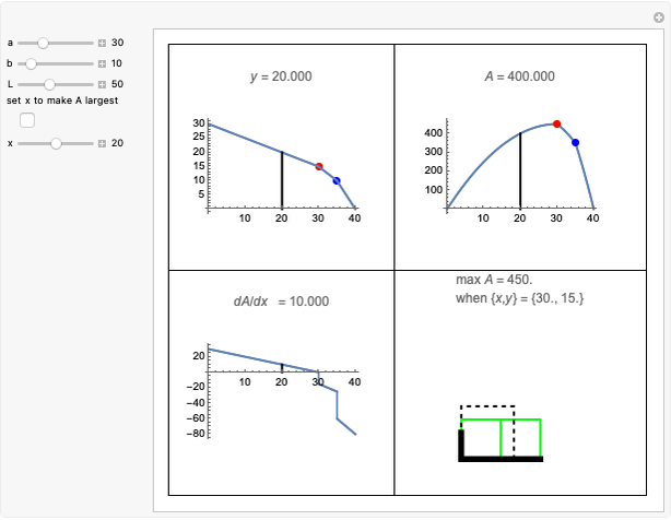 Maximum Area Field with a Corner Wall
Roger B. Kirchner