Underwater Vehicle Pressure Signature


Requires a Wolfram Notebook System
Interact on desktop, mobile and cloud with the free Wolfram Player or other Wolfram Language products.
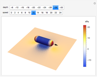
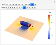
This Demonstration displays the pressure distribution on an idealized underwater vehicle as it moves along near the ocean bottom. The corresponding pressure on the ocean bottom in the vicinity of the vehicle is displayed as well. The ocean is assumed to be an incompressible, inviscid (frictionless) medium with a fixed, rigid bottom. Potential theory is used to model the fluid flow, and the underwater vehicle is modeled as a moving Rankine solid consisting of a single source-sink pair. The method of images is used to account for the fact that there is no vertical fluid flow at the ocean bottom. As the vehicle moves along, it pushes water out of the way. If the vehicle is near the bottom, then there is higher relative fluid velocity underneath the vehicle than there is at a more distant location. The pressure signature caused by this relative velocity change can be computed by using Bernoulli's theorem.
Contributed by: Marshall Bradley (July 2015)
Open content licensed under CC BY-NC-SA
Snapshots


Details
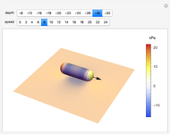
In the Demonstration, the direction of motion of the underwater vehicle relative to the ocean bottom is indicated by the black arrow. The Mathematica ColorGradient "TemperatureMap" has been used to indicate the pressure on the vehicle hull and the ocean bottom. Red and blue correspond to regions of high and low pressure, respectively. Within the Demonstration, the ocean depth has been set to  meters. As the depth of the vehicle approaches the depth of the ocean bottom, water must flow faster beneath the hull. In order to remove time dependence from the problem, the position of the vehicle is held fixed and fluid is moved from left to right at the speed of the vehicle. This produces a pressure-velocity distribution that is equivalent to the vehicle moving through undisturbed fluid. This trick produces a great simplification in the mathematics required to model the problem.
Bernoulli's equation provides a relationship between pressure, the speed of the vehicle, and the velocity of the fluid flow in the water column produced by the motion of the vehicle. In this particular case, Bernoulli's equation takes the form
 ,
,
where  is the pressure at the point
  in the water column,
  is the density of sea water (
 ),
),  is the vector velocity in the ocean caused by the motion of the vehicle,
  is the speed of the vehicle,
  is the acceleration due to gravity,
  is atmospheric pressure, and
  is depth below the ocean surface. A negative value of the depth indicates that the location is beneath the ocean surface. The pressure produced by the motion of the vehicle relative to the hydrostatic pressure
  can be found by rearranging Bernoulli's equation. The result is
 .
.
At a location distant from the position of the vehicle,  and the relative pressure
  is zero. At a location beneath the vehicle and above the ocean bottom,
  is greater than
  and the relative pressure is negative. In order to compute the relative pressure , it is necessary to know the fluid velocity . This velocity can be found by using potential theory to solve the equations of motion governing hydrodynamic flow.
There are three fundamental equations that govern the flow of inviscid fluid. They are the Euler equation, the equation of continuity, and an equation of state. The Euler equation results from applying Newton's second law to the motion of a fluid particle. It is
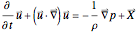 ,
,
where  is body force per unit mass and
  is the gradient operator. The equation of continuity is an expression of conservation of mass. It is
 .
.
An equation of state is an equation of the form
 .
.
An example of an equation of state would be a gas law for an adiabatic process, in the form  , where
  , , and
  are constants.
The preceding three equations provide a total of five independent scalar equations for the five unknowns:  , , and
  . In order to obtain an analytic solution to these equations, we make three simplifying assumptions. First of all, the density is assumed to be the constant
  . This is the same thing as assuming that the fluid is incompressible. Second, we assume that the flow is steady. This assumption results in the simplification
  . And finally, we assume that the flow is irrotational. This last assumption lets us write the vector fluid velocity
  in the form
 .
.
With these three assumptions, the Euler equation can be integrated to yield the first Bernoulli equation shown above. The equation of continuity becomes
 ,
,
which is Laplace's partial differential equation. In principle, a solution to a fluid flow problem under these three simplifying assumptions can be obtained by finding solutions to Laplace's equation that satisfy the relevant boundary conditions. For a rigid ocean bottom, the appropriate boundary condition is that the vertical component of the fluid velocity  .
.
Solutions to Laplace's equation are referred to as potential functions. A fundamental potential function of great importance is a point source of strength  . In mathematical terms it is
 .
.
The fluid velocity field associated with this potential function is
 .
.
The fluid field consists of spherically symmetric flow from the source location. The magnitude of this flow decays like  . If the sign of is reversed, the source becomes a sink. In an infinite medium, a solid body of revolution held fixed with fluid flowing past it parallel to its axis of symmetry can be represented by using combinations of sources and sinks superimposed on a uniform flow at a speed . If only one source and one sink are used, then the body has the shape of a cylinder with spherical end caps. In general, such a body is referred to as a Rankine solid, and in this simple case the appropriate potential function is
 .
.
If the total length of the body is denoted by  and the radius of the spherical end cap is denoted by
  , then in order to achieve the correct shape of the Rankine solid, it is necessary to choose
  and
and  . These two choices place points of stagnation at either end of the solid.
The effect of having a rigid boundary at the depth  can be incorporated into the solution by placing image sources at the depth
  . This leads to the solution
 .
.
If you look closely at the pressure distributions on the fore and aft of the vehicle, you will notice that they appear symmetrical. In the absence of a boundary, they are exactly symmetrical. In this case, the pressure symmetry implies that there is no net force from the flow acting on the vehicle and the motion of the vehicle produces no drag. This flies in the face of common experience and produces a problem for potential flow known as the paradox of d'Alembert. The paradox results from the fact that we did not include frictional effects in the Euler equations. The solution presented here does, however, do a good job of estimating the pressure distribution on the ocean bottom produced by the motion of the vehicle.
References
[1] G. Falkovich, Fluid Mechanics: A Short Course for Physicists, Cambridge: Cambridge University Press, 2011.
[2] H. Jeffreys, Cartesian Tensors, Cambridge: Cambridge University Press, 1965.
[3] G. Polya and G. Latta, Complex Variables, New York: John Wiley & Sons, Inc., 1974.
[4] L. Prandtl and O. G. Tietjens, Fundamentals of Hydro- and Aeromechanics, Mineola, NY: Dover Publications, 1934.
Permanent Citation
 Wilhelmy Plate Apparatus for Measuring Surface Tension
Catherine Lu The Radiation Pressure of Light
Sándor Kabai Micro-Doppler Sonar Simulation
Marshall Bradley Human Walking Animation
Marshall Bradley Active Shock Absorbers
Enrique Zeleny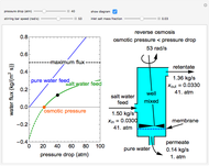 Reverse Osmosis
Muqbil Alkhalaf and Rachael L. Baumann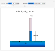 Manometers
Rachael L. Baumann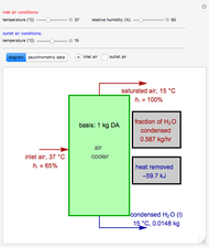 Operation of an Air Conditioner
Housam Binous and Ahmed Bellagi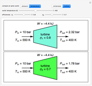 Compare Compressors or Turbines with Different Efficiencies
Rachael L. Baumann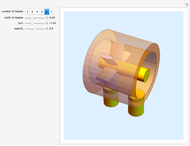 Underwater Turbine
Eider Domínguez
-
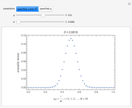
 Bayesian Distribution of Sample Mean
Marshall Bradley -
 Fluid Flow around a Corner
Marshall Bradley -
 Underwater Vehicle Pressure Signature
Marshall Bradley -
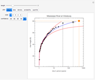 Extreme Value Forecasting
Marshall Bradley -
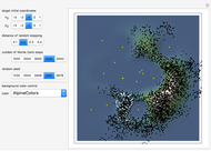 Target Motion with the Metropolis-Hastings Algorithm
Marshall Bradley -
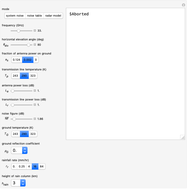 Noise Temperature of a Radar System
Marshall Bradley -
 High-Frequency Sonar Performance
Marshall Bradley -
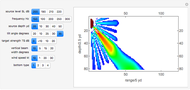
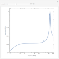 Atmospheric Radar Wave Absorption
Marshall Bradley -
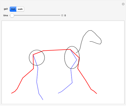 Equine Motion
Marshall Bradley -
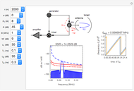 Frequency-Modulated Continuous-Wave (FMCW) Radar
Marshall Bradley -
 Maximum Entropy Probability Density Functions
Marshall Bradley -
 Uncertainty in Sonar Performance Prediction
Marshall Bradley -
Micro-Doppler Sonar Simulation
Marshall Bradley -
Human Walking Animation
Marshall Bradley -
 Bayesian Range Weighting for Sonar
Marshall Bradley