Meshless Approximation


Requires a Wolfram Notebook System
Interact on desktop, mobile and cloud with the free Wolfram Player or other Wolfram Language products.
Meshless approximation methods make possible the definition of a continuous function that approximates a set of values at any point  in the domain
  . The approximation function is defined as
  , where
 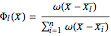 with
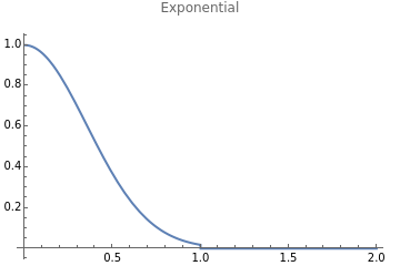
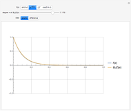
with  a weight function that depends on the radius of influence, that is, it is a radial basis function (RBF). Typical weight functions are an exponential, a cubic or quartic spline, or SPH (smoothed particle hydrodynamics). Some of them can be customized with the smoothness parameter
  .
.
Contributed by: Enrique Fernández Perdomo (March 2011)
Suggested by: José M. Escobar Sánchez
Open content licensed under CC BY-NC-SA
Snapshots


Details
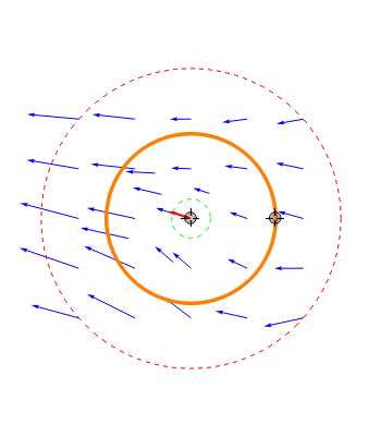
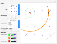
The right graphic shows data samples as a vector field with blue arrows and a locator to get the approximation at any point within the domain , represented by a red arrow. Three circles represent the minimum radius (dashed green), maximum radius (dashed red), and current radius (orange), which determine the samples used to compute the approximation. You can use the other locator to modify the current radius between the minimum and maximum radius ranges, which take only one sample and all samples, respectively.
The controls on the left are divided into three sections. The samples section lets you choose the samples dataset to work with. The approximation section has a pair of sliders that let you configure the current radius and smoothness parameter . The range of the parameter depends on the weight function selected; it is disabled for the cubic and quartic splines. The current approximation position and value are shown numerically. Finally, the appearance section lets you change the minimum radius, maximum radius, and current radius and the circles' colors. Moreover, there are tooltips for the circles and the locator in the right graphic to show their current values.
Further background regarding meshless methods and weight functions used is provided by (Belytschko, 1996).
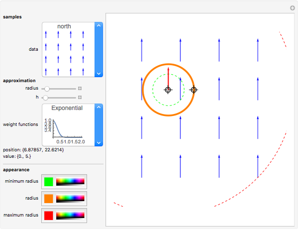
Snapshot 1: when all samples have the same value (e.g., dataset north), the approximation value is the same at every point
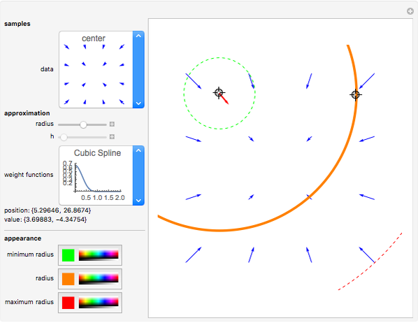
Snapshot 2: different weight functions produce slightly different approximation values with the same radius and smooth parameter ; the cubic and quartic spline do not depend on
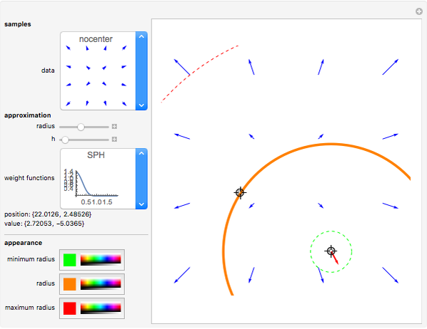
Snapshot 3: the SPH weight function depends on the smooth parameter . Though the function shape is constant, the scale in both axes is not. The exponential weight function depends on , too, but its shape varies from the Dirac delta to the Heaviside step function.
Snapshot 4: the smoothness parameter for the SPH weight function must be greater than  , so the minimum allowed value is set to
  , where
  . Lower values would produce a null approximation value.
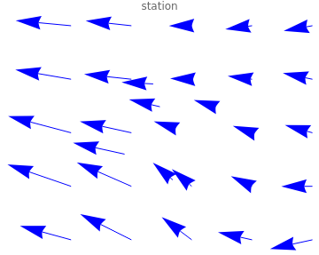
Snapshot 5: the station dataset is taken from real weather stations (wind rate). With radius close to the minimum allowed value, the approximation is similar to the closest sample.
Snapshot 6: with the radius close to the maximum, all samples will be taken into account depending on the parameter
Snapshot 7: with smaller , the approximation is more similar to the closest sample
Snapshot 8: with larger , the approximation is less similar to the closest sample. With  , the approximation tends to the sample's mean, independently of the position. Better values are those lower than 1.
Permanent Citation
 Weierstrass Approximation Theorem
Fabián Alejandro Romero Gauss-Legendre Approximation of Pi
Russ Johnson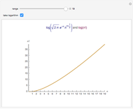 Stirling's Approximation versus n!
Sam Nicoll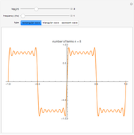 Approximation of Discontinuous Functions by Fourier Series
David von Seggern (University Nevada-Reno)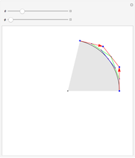 Bézier Curve Approximation of an Arc
Rob Raguet-Schofield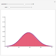 Normal Approximation to a Poisson Random Variable
Chris Boucher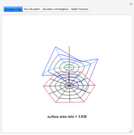 Series Approximation for the Schwarz D Surface
Brad Klee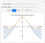 Padé Approximants
Oleksandr Pavlyk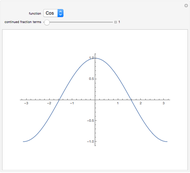 Continued Fraction Approximations
Michael Trott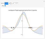 Multipoint Padé Approximants
Blazej Radzimirski
