Quantum Motion of Two Particles in a 3D Trigonometric Pöschl-Teller Potential


Requires a Wolfram Notebook System
Interact on desktop, mobile and cloud with the free Wolfram Player or other Wolfram Language products.
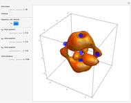
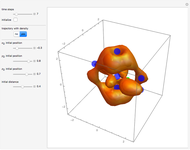
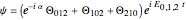
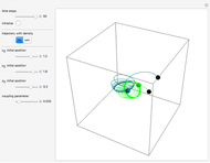
Exact solutions of the nonrelativistic wave equations contain all the necessary information for the quantum system and have important applications in particle physics. This Demonstration discusses a solution of the Schrödinger equation in three-dimensional configuration space with the trigonometric Pöschl–Teller potential in the Bohm approach.
[more]

Contributed by: Klaus von Bloh (March 2015)
Open content licensed under CC BY-NC-SA
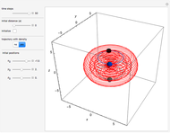
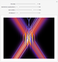
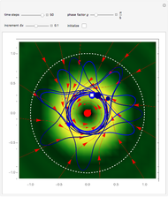
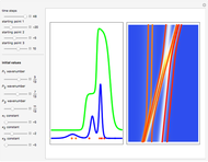
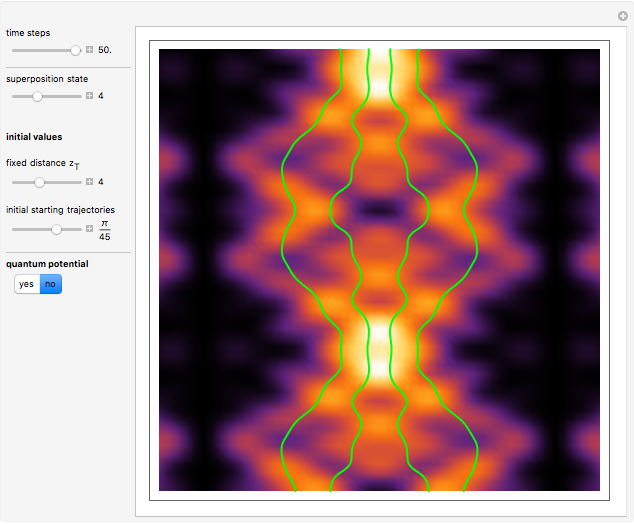
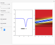
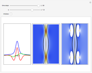
Snapshots


Details
Associated Legendre polynomials arise as the solution of the Schrödinger equation:
 ,
,
with the integers  ,
,  ,
,  ,
,  , and so on. A degenerate, unnormalized wavefunction
  with time period
  for
for  for the three-dimensional case can be expressed by:
 ,
,
where  ,
,  ,
, 
 are eigenfunctions, and
  are permuted eigenenergies of the corresponding stationary one-dimensional Schrödinger equation with
  . The eigenfunctions are defined by
 ,
,
where  ,
,  ,
,  are associated Legendre polynomials. The parameter
  is a constant phase shift , and are the quantum numbers
  with
with  and
and  . The wavefunction is taken from [2].
For this Demonstration, the wavefuction is defined by:
 .
.
Due to the permuted wavefunction structure and depending on the constant phase shift , most of the nodal points are positioned only in the  ,
,  plane.
The velocity field  is calculated from the gradient of the phase from the total wavefunction in the eikonal form (often called polar form)
  . The time-dependent phase function
  from the total wavefunction is:
 , with
 .
.
The corresponding velocity field becomes time independent (autonomous) because of the gradient of the phase function.
The velocity in the direction becomes zero if  , which is fulfilled for
  . The velocities in the other directions become zero for
  . The length of the curve depends on the constant phase shift .
In the program, if PlotPoints, AccuracyGoal, PrecisionGoal, and MaxIterations are increased, the results will be more accurate.
References
[1] G. Pöschl, E. Teller, "Bemerkungen zur Quantenmechanik des anharmonischen Oszillators," Zeitschrift für Physik, 83 (3–4), 1933 pp. 143–151. doi:10.1007/BF01331132.
[2] M. Trott, The Mathematica GuideBook for Symbolics, New York: Springer-Verlag, 2006.
[3] "Bohmian-Mechanics.net." (Mar 16, 2015) www.bohmian-mechanics.net/index.html.
[4] S. Goldstein. "Bohmian Mechanics." The Stanford Encyclopedia of Philosophy. (Mar 16, 2015)plato.stanford.edu/entries/qm-bohm.
[5] K. von Bloh. The Quantum Motion of Eight Particles in a 3D Trigonometric Pöschl–Teller Potential. [Video]. (Mar 16, 2015) www.youtube.com/watch?v=ejJF3cSWa4Y.
Permanent Citation
 Chaotic Quantum Motion of Two Particles in a 3D Harmonic Oscillator Potential
Klaus von Bloh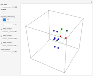 Periodic Quantum Motion of Two Particles in a 3D Harmonic Oscillator Potential
Klaus von Bloh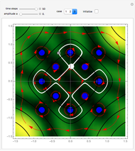 Bohmian Quantum Trajectories for Coherent States of the Pöschl-Teller Potential
Klaus von Bloh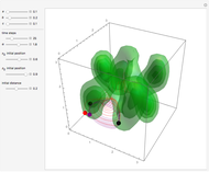 Bohm Trajectories for a Particle in an Infinite 3D Box
Klaus von Bloh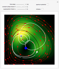 Bohm Trajectories for a Particle in a Two-Dimensional Calogero-Moser Potential
Klaus von Bloh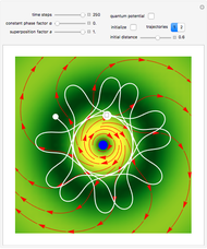 Bohm Trajectories for the Two-Dimensional Coulomb Potential
Klaus von Bloh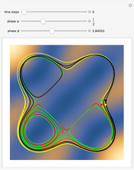 Simple Chaotic Motion of Quantum Particles According to the Causal Interpretation of Quantum Theory
Klaus von Bloh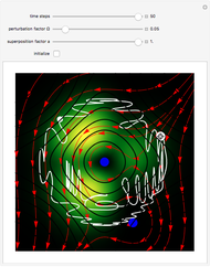 Perturbation Theory in the de Broglie-Bohm Interpretation of Quantum Mechanics
Klaus von Bloh Bohm Trajectories for Quantum Particles in a Time-Dependent Linear Potential
Klaus von Bloh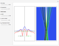 Continuous Transition between Classical and Bohm Quantum Pictures for Young's Interference Experiment
Partha Ghose and Klaus von Bloh
-
Bohm Trajectories for the Two-Dimensional Coulomb Potential
Klaus von Bloh -
 Bohm Trajectories in an LCAO Approximation for the Hydrogen Molecule H_2
Klaus von Bloh -
 Decoherence and Trajectories Implied by a Modified Schrodinger Equation
Klaus von Bloh -
 Bohm Trajectories for a Particle in a Two-Dimensional Circular Billiard
Klaus von Bloh -
 From Bohm to Classical Trajectories in a Hydrogen Atom
Klaus von Bloh -
 Continuous Transition between Quantum and Classical Behavior for a Harmonic Oscillator
Klaus von Bloh -
Continuous Transition between Classical and Bohm Quantum Pictures for Young's Interference Experiment
Klaus von Bloh -
 Bohm Trajectories for Quantum Particles in a Uniform Gravitational Field
Klaus von Bloh -
Bohm Trajectories for a Particle in a Two-Dimensional Calogero-Moser Potential
Klaus von Bloh -
 Nonlocality in the de Broglie-Bohm Interpretation of Quantum Mechanics
Klaus von Bloh -
 Three-Soliton Collision in the Trajectory Approach
Klaus von Bloh -
 The Which-Way Experiment and the Conditional Wavefunction
Klaus von Bloh -
Chaotic Quantum Motion of Two Particles in a 3D Harmonic Oscillator Potential
Klaus von Bloh -
Perturbation Theory in the de Broglie-Bohm Interpretation of Quantum Mechanics
Klaus von Bloh -
Periodic Quantum Motion of Two Particles in a 3D Harmonic Oscillator Potential
Klaus von Bloh -
 Quantum Motion of Two Particles in a 3D Trigonometric Pöschl-Teller Potential
Klaus von Bloh -
 The Talbot Carpet in the Causal Interpretation of Quantum Mechanics
Klaus von Bloh -
Bohmian Quantum Trajectories for Coherent States of the Pöschl-Teller Potential
Klaus von Bloh -
 Gray and Dark Solitons in the de Broglie and Bohm Approaches
Klaus von Bloh -
 A Breather Solution in the Causal Interpretation of Quantum Mechanics
Klaus von Bloh