Random Simulation of a Financial Portfolio

Requires a Wolfram Notebook System
Interact on desktop, mobile and cloud with the free Wolfram Player or other Wolfram Language products.
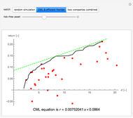
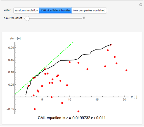
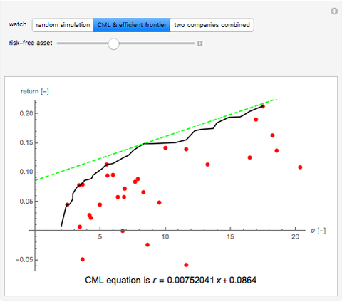
This Demonstration uses random number generation to create a portfolio with up to 30 elements (represented by red points) taken from the Dow Jones Industrial Average using data from 2003 to 2010. The yellow point shows a portfolio with weight 1/30 for each asset. The program finds the efficient frontier according to modern portfolio theory and shows the capital market line (CML) from the 1500 generated points. The CML consists of the risk-free asset's return and market portfolio lying on the efficient frontier. The combination of the two companies shows possible trajectories of the portfolio according to the correlation.
Contributed by: Alois Neumann (September 2011)
(Czech Technical University)
Open content licensed under CC BY-NC-SA
Snapshots


Details
A random simulation is faster than an analytical solution, which also takes too much memory. Every blue point is defined by the equations 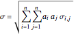 and
and  , where
  are the contributions of asset
  ,
,  ,
,  to a portfolio,
  is the covariance of assets
  and
and  ,
,  is the expected return of asset
  . The second control, "CML & efficient frontier", finds the efficient frontier, which consists of all the points that give the best return at the same level of volatility and the curve is nondecreasing. The more points we use for the simulation, the smoother the efficient frontier. The efficient frontier is necessary for finding the CML. A CML is defined by equation
  . Here
  is the expected return,
  is the risk-free return,
  is the slope of the line, and
  is the volatility. The only unknown element is
  , but we know that CML is tangent to the efficient frontier; the highest possible slope of the line is defined by two points: a risk-free return and a point on the efficient frontier. The third control "two companies combined" shows a trajectory of a portfolio that is composed of two companies. Every point of the trajectory is defined by equations
  and
and  , where
  is the contribution of asset 1 to a portfolio,
  is the contribution of asset 2 to a portfolio,
  is the expected return of asset 1,
  is the expected return of asset 2,
  is the volatility of the portfolio,
  is the variation of asset 1,
  is a variation of asset 2, and
  is the covariance of assets 1 and 2. Here
  ,
,  , with the restriction
  .
.
Permanent Citation
"Random Simulation of a Financial Portfolio"
http://demonstrations.wolfram.com/RandomSimulationOfAFinancialPortfolio/
Wolfram Demonstrations Project
Published: September 16 2011
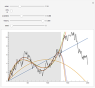 Polynomial Fits of Random Walks
Michael Schreiber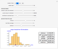 Monte Carlo Simulation of Retirement Savings with Variable Annual Return
Paul Savory (University of Nebraska-Lincoln) Bootstrapping Credit Default Swap Data
Jeff Hamrick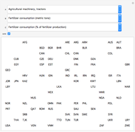 World Bank Data Series Overview
Michael Schreiber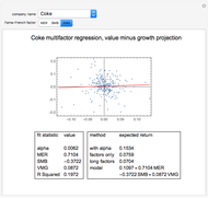 Expected Returns of the Dow Industrials, Fama-French Model
Jeff Hamrick and Jason Cawley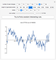 Minimal Model of Simulating Prices of Financial Securities Using an Iterated Finite Automaton
Philip Maymin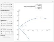 Kelly Portfolio Analysis
Stephen Schulist Trader Dynamics in Minimal Models of Financial Complexity
Philip Maymin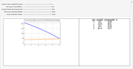 Fund Drawdown Simulation
Joe O'Hara Markov Volatility Random Walks
Jason Cawley
