Graphics Lighting Transformation


Requires a Wolfram Notebook System
Interact on desktop, mobile and cloud with the free Wolfram Player or other Wolfram Language products.
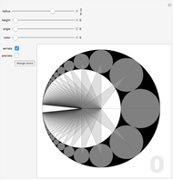
A sphere can be transformed into a spheroid by either a scale transformation or by changing the plot range while keeping the bounding box ratios constant. These transformations are specified by the spheroid control setting, which gives the vertical over horizontal semi-axis ratio of the resulting spheroid. A control setting less than 1 gives an oblate spheroid, greater than 1 a prolate spheroid, and equal to 1 an untransformed sphere.
[more]
Contributed by: Christopher Haydock (February 2013)
(Applied New Science LLC)
Open content licensed under CC BY-NC-SA
Snapshots


Details
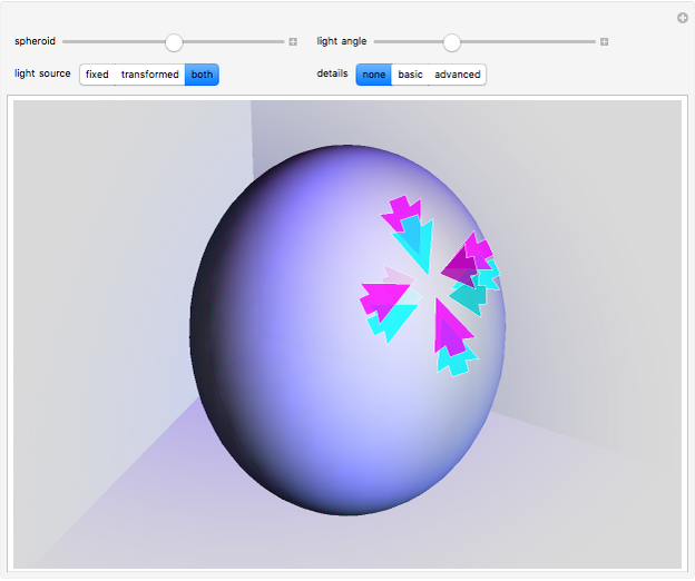
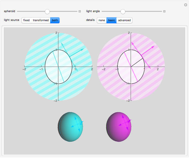
The details setter bar selects the main view (snapshot 1) and the basic and advanced detail views (snapshots 2 and 3), which show 2D cross-sections defined by the intersection of the vertical spheroid symmetry axis and the lighting direction. The left side of the basic view shows the fixed cyan light source and the spheroid generated by a scale transformation. The right basic view shows the transformed magenta light source and the spheroid generated by changing the plot range. The left and right cross-sections also indicate the normal incidence points and terminators for the cyan and magenta light sources. As the spheroid control is varied, it is evident that the left axis labels, plot range, and cyan lighting direction remain constant because this spheroid transformation involves only scaling the sphere, whereas the right axis labels and magenta light direction vary continuously with the spheroid setting because this spheroid transformation changes the plot range. Finally, the black radial vector on the right basic view is useful for visual confirmation that the magenta light source is a constant before transformation. As the spheroid control moves through the oblate range, it is possible to visualize a 3D disk rotating about the horizontal axis and imagine that the radial vector is fixed on the disk, and likewise in the prolate range to visualize a 3D disk with fixed radial vector rotating about the vertical axis.
The advanced details view (snapshot 3) further elaborates the basic view's left side scale and right side plot range sphere to spheroid transformations. The right side advanced view doesn't actually include the plot range transformation; instead it shows the sphere cross-section, light sources, normal incidence points, and terminators before applying the plot range transformation. The sphere cross-section is just that, and the magenta light source simply needs to be fixed at the angle defined by the light angle control and its terminator is perpendicular to this angle. The magenta light source is referred to as the transformed light source precisely because it naturally undergoes the same sphere to spheroid transformation created by changing the plot range at constant bounding box ratios. Of course, the point of normal incidence of the magenta light on the spheroid is not simply given by transforming its point of normal incidence on the sphere. Furthermore the direction and length of the arrows marking the point of normal incidence must be so constructed that they are of correct length and tangent or normal after the plot range transformation. As is immediately evident in the advanced details view, it also differs from the basic details view in that both the cyan and magenta light sources are shown on both the left and right side of the view. For example, the left side advanced view starts with the basic view fixed cyan source and adds the transformed magenta light source. Because all objects and light sources on the left side are individually scaled, this means that the sphere to spheroid transformation must be manually applied to the magenta source as already described above in the main view caption: "the magenta light source direction is determined by applying the spheroid transformation to a lighting direction vector with an inclination angle specified by the light angle control." The right side advanced view essentially swaps the lighting procedure. It starts with the basic details view transformed magenta source, but this source is fixed at the inclination angle specified by the light angle control and does not rotate with changes in the spheroid control because the right advanced view shows everything before applying the plot range transformation. To add the fixed cyan source, the inverse sphere to spheroid transformation must be applied to a lighting direction vector with an inclination angle specified by the light angle control. Thus on the right side of the advanced details view, the magenta light source will be fixed and the cyan source will be seen to rotate as the spheroid control setting is changed.
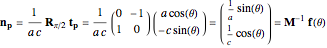
All the transformations appearing in the source code are derived from the following definitions and equations. A point on the elliptical cross-section through the vertical symmetry axis of a spheroid can be simply parameterized by the angle  , such that a point
  is given by the action of a positive valued diagonal matrix
  on a unit angle vector
  :
:
 ,
,  ,
,  ,
,  .
.
The unit angle vector  component is given by
  and the
  component by
  because the inclination angle is measured from the vertical. The diagonal components of the matrix are the spheroid equatorial radius
  and polar radius
  , or equivalently, the ellipse horizontal radius and vertical radius . A normal vector at a point is given by a 90° rotation of the point vector partial derivative with respect to the parameter:
 ,
,  ,
,
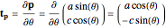 .
.
The scale factor  sets the normal vector exactly equal to the action of the inverse diagonal matrix
  on the unit angle vector and makes explicit the symmetry of a spheroid point and its normal, which are respectively generated by the action of the diagonal matrix and its inverse on the angle vector. The above normal vector equation essentially gives a relation between the light angle and the point of normal incidence. To complete this relation, let curly
  be the light inclination angle from vertical and set the corresponding unit angle vector
  equal to the normalized normal vector:
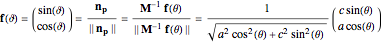 .
.
Given a parameterized point on a spheroid, this equation gives the light angle that is normally incident on that point. In practice we usually want the inverse angle relation, that is, given the light angle curly find the normal incidence point angle parameter plain . The inverse relation is easily derived by left-multiplying both sides of the above curly equation by the diagonal matrix and normalizing:
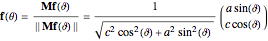 .
.
For more on Lambertian diffuse reflections, see the Mathematica tutorial "Lighting and Surface Properties".
Permanent Citation
 Image Smoothing Using Stationary Wavelet Transform
Stefan Ganev 3D Graphics with 2D Overlay
Yuzhu Lu and Chris Hill Colored Lights
Jeff Bryant Text Positioning in Three Dimensions with Nested Transformations
Chris Hill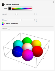 Diffuse and Specular Reflection
Christopher Haydock (Applied New Science LLC)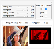 Selecting from ImageData Using Rows and Columns
Nasser M. Abbasi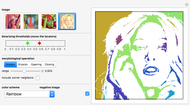 Creating Posters from Photographic Images
Erik Mahieu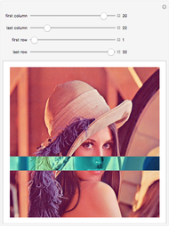 Image Processing on Partitions
Nick Lariviere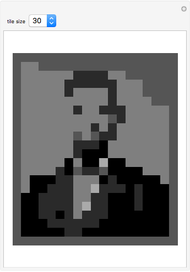 Guess Who?
Ken Levasseur (UMass Lowell)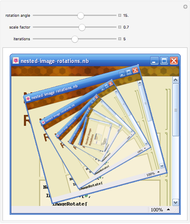 Nested Image Rotations
Robert Dickau