Capacity Planning for Short Life Cycle Products: The Newsvendor Model


Requires a Wolfram Notebook System
Interact on desktop, mobile and cloud with the free Wolfram Player or other Wolfram Language products.
The newsvendor model is classically used for inventory (equivalently "capacity") management of short life cycle or perishable products such as fashion goods, electronics, and so on, but it can also be used to aid long-term strategic capacity investment. The key idea is to acquire capacity in the face of unknown demand by balancing the expected cost of ordering too little versus the cost of ordering too much. When demand increases, it is then satisfied contingent upon the acquired capacity. The newsvendor model is also one of the basic examples of stochastic programming with recourse and represents a real options type of approach. In the example shown, demand is modeled using the Gaussian distribution, although you can use the newsvendor model with any continuous or discrete distribution, and even if you know only the mean and standard deviation of an otherwise unknown distribution.
Contributed by: Shailesh S. Kulkarni (March 2011)
Based on a program by: Chris Boucher
Open content licensed under CC BY-NC-SA
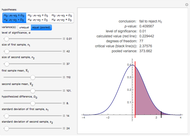
Snapshots

Details
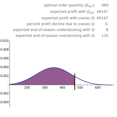
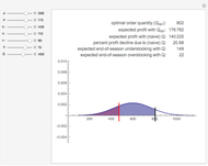
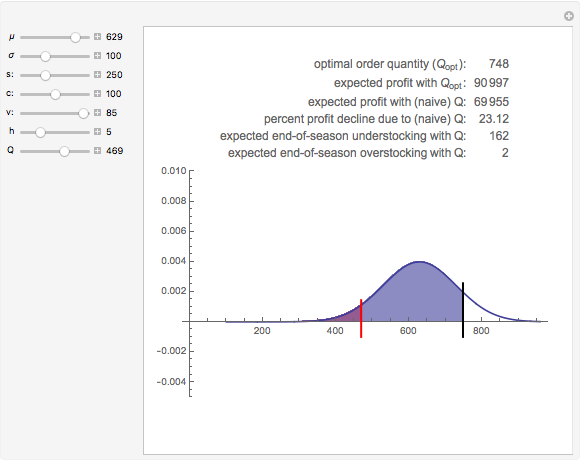
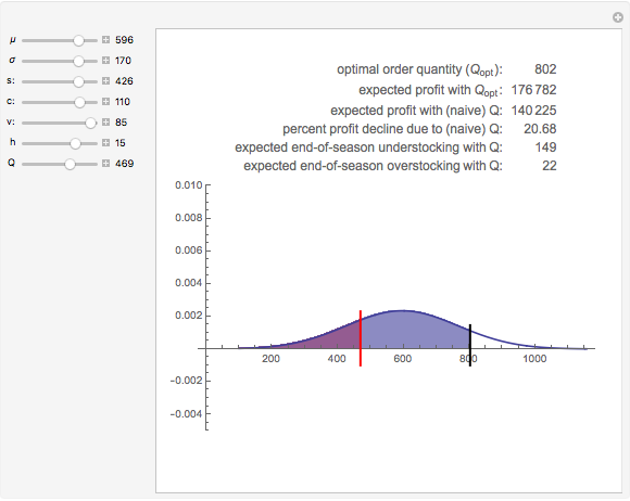
Although the newsvendor model in its very basic form involves a single product and a single period, it has been extended to multiple products, multiple processing points, and multiple periods. It is then referred to as a "newsvendor network". In addition, the risk aversion of decision makers can be incorporated into the basic and extended models. All these extensions, though, come at the expense of analytic tractability. However, numerical solutions are not too difficult to calculate even for large newsvendor networks, given the large-scale optimization engines available today. The analytic formula for the basic newsvendor model (for a continuous demand distribution) is to order at the critical fractile that equals 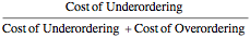 . Note that in the example presented here this works out to be
  =
= =0.88235. Upon inverting the cumulative distribution function of the distribution (N(350, 100)) at this critical fractile we get the optimal order quantity of 469 as depicted in the Demonstration. When the demand distribution is discrete, one should order the smallest quantity at which the cumulative distribution equals or exceeds the critical fractile.
 : average (mean) demand
 : standard deviation of demand
 : unit selling price
 : unit purchase cost
 : unit markdown price for unsold items
 : unit holding cost for unsold items
 : naive (or heuristic) order quantity
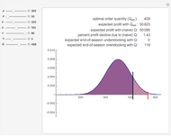
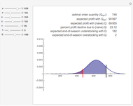
Snapshot 1: notice what happens when the demand distribution has less variance
Example from: S. Chopra and P. Meindl, Supply Chain Management, Pearson Higher Education, 2007.
Permanent Citation
 Monopoly Model
David Youngberg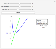 Competitive Model
David Youngberg Simple Solow Model
Alex Tabarrok An Inventory Control Model
Chris Boucher A Simple Inventory Control Model
Chris Boucher The Paradox of Thrift in a Simple Stock-Flow Consistent Model
Kevin W. Capehart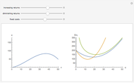 Short-Run Production and Cost Curves
Tom Creahan Hotelling Model of Product Quality Differentiation
Timur Gareev Short-Run Cost Curves
William J. Polley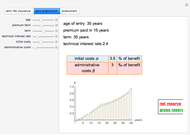 Net and Gross Reserve of Life Insurance
Gergely Nagy