Digital IIR Filter Design Showing Poles and Zeros


Requires a Wolfram Notebook System
Interact on desktop, mobile and cloud with the free Wolfram Player or other Wolfram Language products.
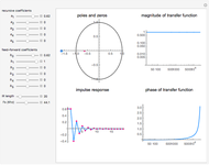
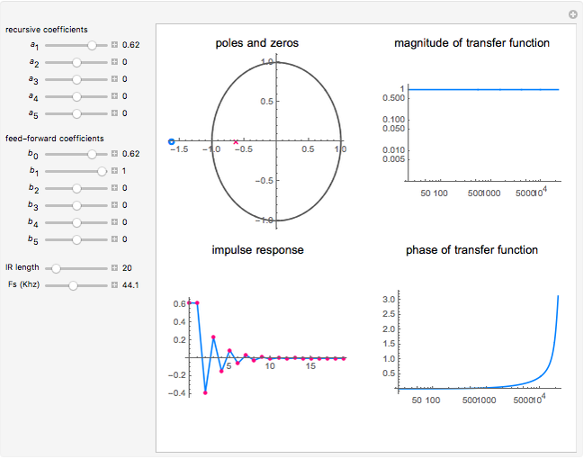
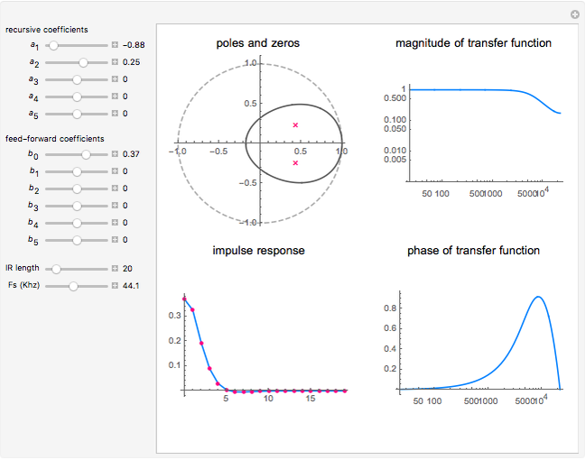
This Demonstration visualizes properties of a general fifth-order digital infinite impulse response (IIR) filter specified by the following expansion:
[more]


Contributed by: Hans Anderson (August 2015)
Open content licensed under CC BY-NC-SA
Snapshots

Details
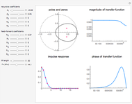
Snapshot 1: first-order all-pass filter
Snapshot 2: all-pole filter reducing amplitude of high frequencies
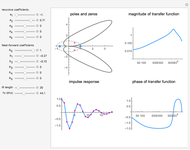
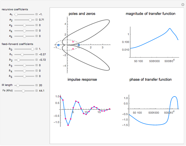
Snapshot 3: bandpass filter
The transfer function of the general fifth-order digital IIR filter as shown in this Demonstration is represented by
 .
.
Given an input  , the output of the filter,
  , is determined by
  . Thus, the transfer function for the filter specifies the change in amplitude and phase on an input with frequency distribution defined by the unitary complex number
  . For example, if the magnitude of the transfer function at frequency
  is 0.5, then the filter output amplitude at that frequency will be half the amplitude of the input.
In filter design, it is helpful to know which complex valued inputs to the transfer function produce zero output amplitude and which inputs produce infinite output amplitude. This information is readily available by examining the numerator and denominator of the transfer function. Specifically, if for a given input value the numerator is zero, then the entire transfer function evaluates to zero. Likewise, if for  the denominator is zero, then the value of the transfer function is infinite. Complex values of for which
  are called zeros of the transfer function, while values for which is infinite are called poles.
When we plot the transfer function of a digital filter, we let  and generate the plot by varying in the range
  . In this way, we cover the entire range of frequencies from 0 up to the Nyquist frequency, which is half the sampling rate. Hence the value
  indicates the maximum frequency at which the filter operates without aliasing.
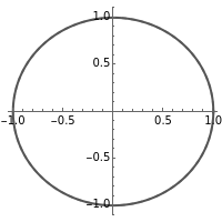
In this Demonstration, the poles and zeros plot shows the location of the poles and zeros in the complex plane. For a benchmark, the unit circle is also shown with a dashed line. The solid line shows the absolute value of the transfer function plotted in polar coordinates as the angle varies from  to
to  and from to
  .
.
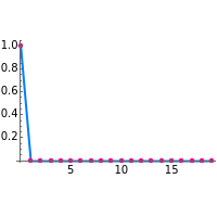
The impulse response plot shows the individual sample values that would result from applying the digital filter to an input containing a single one followed by zeros:  . This is useful for illustrating how the filter causes impulsive inputs to spread out in the time domain.
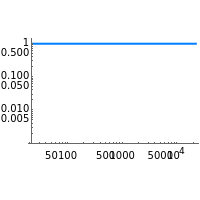
The magnitude and phase plots show  and
and  , respectively, plotted with
  so that the frequency ranges from up to , which are the minimum and maximum frequencies representable in a digital system.
Reference
[1] R. Allred, Digital Filters for Everyone: Third Edition, Creative Arts & Sciences House, 2015.
Permanent Citation
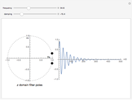 Sine Wave Generation Using an Unstable IIR Filter
Charles Masenas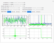 Digital Filters with Windowed Sinc Finite Impulse Response
Dana Tremblay Comparing Two Discrete Lowpass Filters with Low Distortion
Ted Ersek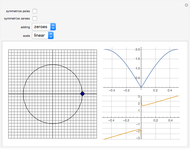 Transfer Function from Poles and Zeroes
Philippe Thévenaz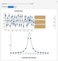 Bit Response of a PR4 Encoded Magnetic Medium
Charles Masenas Infinite Impulse Response (IIR) Digital Low-Pass Filter Design by Butterworth Method
Nasser M. Abbasi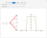 Lowpass Filter Design by Pole Placement
Aaron T. Becker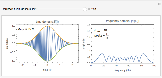 Spectral Broadening Induced by Self-Phase Modulation
Ruibo Jin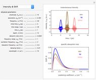 Optical Properties of Biological Tissue in the THz Radiation Regime
Muhamad Hamdi and Yusof Munajat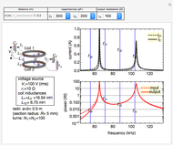 Wireless Power Transmission
Y. Shibuya