Ikeda Delay Differential Equation


Requires a Wolfram Notebook System
Interact on desktop, mobile and cloud with the free Wolfram Player or other Wolfram Language products.
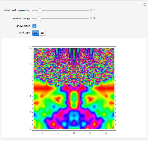
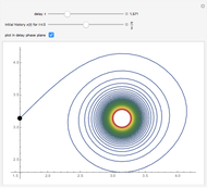
This Demonstration shows solutions of the Ikeda delay differential equation,  , a very simple equation with complex chaotic dynamics.
Contributed by: Rob Knapp (March 2011)
Open content licensed under CC BY-NC-SA
Snapshots


Details
A form of the equation was first proposed to model an optical bistable resonator system [1]. The route to chaos as  increases to
  is described in [2]. For larger values of the solutions look and behave statistically like Brownian motion.
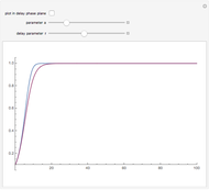
Snapshot 1: just above the value  , where the stable quilibrium changes from a node to a focus
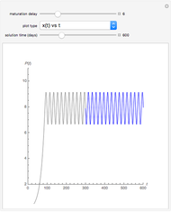
Snapshot 2: just above the value  , at which there is a Hopf bifurcation and the appearance of a limit cycle
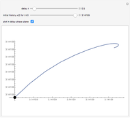
Snapshot 3: just above the value  , at which a pitchfork bifurcation occurs, leading to two coexisting limit cycles
Snapshot 4: the other limit cycle for the same value of ; the initial condition is very close to that of snapshot 3
Snapshot 5: just above the value  , at which a period doubling occurs
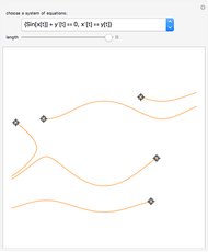
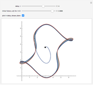
Snapshot 6: just above the value , where chaos first occurs; note how the solution looks much like Brownian motion
Snapshot 7: just above the value  where a periodic window appears
[1] K. Ikeda and K. Matsumoto, "High-Dimensional Chaotic Behavior in Systems with Time-Delayed Feedback," Physica D, 29, 1987 p. 223.
[2] J. C. Sprott, "A Simple Chaotic Delay Differential Equation," Physics Letters A, 366, 2007 pp. 397–402.
Permanent Citation
 Mackey-Glass Equation
Rob Knapp Double Pendulum
Rob Morris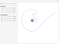 Lorenz Attractor
Rob Morris Pen Falling Off a Finger
Michael Trott Forced Oscillator with Damping
Rob Morris Nonlinear Wave Equations
Stephen Wolfram and Rob Knapp Visualizing the Solution of Two Linear Differential Equations
Mikhail Dimitrov Mikhailov Chaos and Order in the Damped Forced Pendulum in a Plane
Francisco Javier Sanchez Chapado Nonlinear Wave Equation Explorer
Stephen Wolfram Mathematics of Tsunamis
Yu-Sung Chang