Bounce Time for a Bouncing Ball

Requires a Wolfram Notebook System
Interact on desktop, mobile and cloud with the free Wolfram Player or other Wolfram Language products.
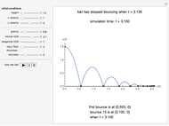
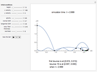
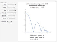
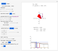
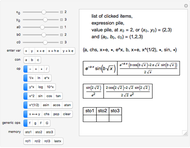
Click "toss the ball" for an animation. Initially, the ball is tossed horizontally with speed 1 m/s from a height of 1.5 m onto a flat floor. The ball has normal and tangential coefficients of restitution of 0.7 and 0.8. (That means the normal and tangential speeds are reduced by factors of 0.7 and 0.8 at each bounce.) It takes 3.10 seconds for the ball to bounce 13 times, and then it has moved horizontally 1.96 m. The formulas below show the ball has finished bouncing at time 3.135, and it is stopped at (1.96, 0).
[more]


Contributed by: Roger B. Kirchner (February 2010)
Based on programs by: Enrique Zeleny, Rob Morris, and Oleksandr Pavlyk
Open content licensed under CC BY-NC-SA
Snapshots


Details
The program for computing the bouncing ball's path is adapted from the bouncing ball example in the Mathematica tutorial "EventLocator" Method for NDSolve, and Enrique Zeleny's Demonstration Stroboscopic Photograph of a Bouncing Ball.
The program for animating the ball is adapted from Rob Morris and Oleksandr Pavlyk's Demonstration Animated Projectile Motion.
The bouncing ball program assumes that if the tangential and normal components of velocity are  and
and  before a bounce, they are
  and
and  after the bounce, where
  . We have generalized so the reflected components are
  and -
and - , where we call
  the tangential coefficient of restitution and
  the normal coefficient of restitution. There may be a reason to assume
  , but
, but  is the usual coefficient of restitution, and
  seems to be a frictional effect. Of course, friction would affect rotation, which we ignore.
Permanent Citation
 Ball Bouncing in a Potential Well
Enrique Zeleny Nonlinearized Motion of a Simple Pendulum
Sarah Lichtblau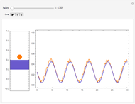 Ball Bouncing on a Moving Piston
Enrique Zeleny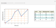 Time-Displacement Plots
Enrique Zeleny Deformation of a Tennis Ball and Racket Strings
Enrique Zeleny Motion of Two Balls Connected by a Rod
Enrique Zeleny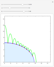 Ball Bouncing on an Elliptical Slope
Housam Binous and Ahmed Bellagi Paths of Balls Bouncing Off Pegs
Abigail Nussey Runge-Kutta versus Velocity-Verlet Solutions for the Classical Harmonic Oscillator
Luigi Tiburzi Multi-Force Newtonian Particle Simulator
Andy P. J. Hanson
-
 Bounce Time for a Bouncing Ball
Roger B. Kirchner -
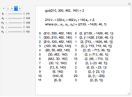
 Generalizing the Crease Length Problem
Roger B. Kirchner -
 Exploring the Crease Length Problem
Roger B. Kirchner -
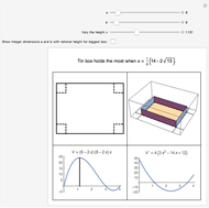 Tin Box with Maximum Volume
Roger B. Kirchner -
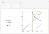
 Automatic Differentiation
Roger B. Kirchner -
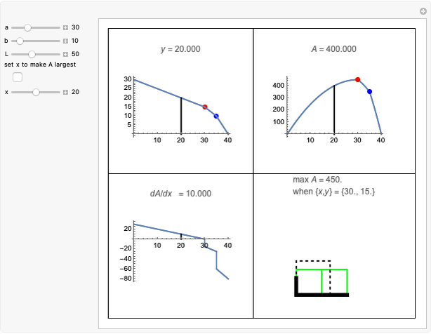 Maximum Area Field with a Corner Wall
Roger B. Kirchner -
 Recursive Extended Euclidean Algorithm
Roger B. Kirchner -
 A Double Exponential Equation
Roger B. Kirchner -
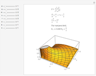 Limits of a Rational Function of Two Variables
Roger B. Kirchner -
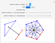 Median Theorem for Polygons
Roger B. Kirchner -
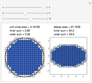 Area of an Ellipse
Roger B. Kirchner -
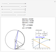 Swim, Swim and Walk, or Walk?
Roger B. Kirchner -
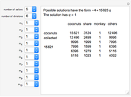 Coconuts, Sailors, and a Monkey
Roger B. Kirchner -
 Pi-Like Ratios for Circular Lakes
Roger B. Kirchner