Component Identification and Boundary Delineation


Requires a Wolfram Notebook System
Interact on desktop, mobile and cloud with the free Wolfram Player or other Wolfram Language products.
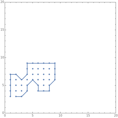
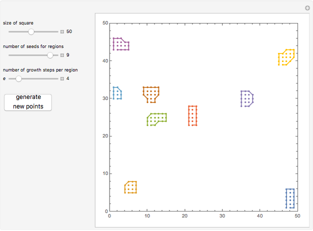
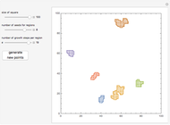
Morphological component identification and boundary delineation are important problems. For a given square grid, based on some thresholding, we want to find the separate components and their boundaries. This Demonstration implements the "one component at a time" marching squares method for the former and the Moore boundary tracing algorithm for the latter. A step before showing this is to first create some artificial regions. For this, the Moore neighborhood is itself used in a nested fashion on a set of seed points.
Contributed by: Raja Kountanya (February 2015)
Open content licensed under CC BY-NC-SA
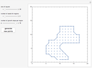
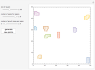
Snapshots


Details
A set of points is given in an  square grid. A Moore window around a point is the list of eight points surrounding it, corresponding to its NW, N, NE, E, SE, S, SW, and W neighbors. To illustrate the component identification and boundary delineation, it is important to construct some artificial components first. To do this, points from the Moore windows of a set of randomly chosen seeds are added to form a new set. Then more points from Moore windows of random points of this set are added. As this process is applied
  times and duplicate copies are deleted each time, the set grows into multiple windows of random shapes.
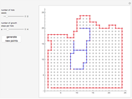
The morphological component identification is performed with the routines BottomLeftPoint, RetWindow, and AllWindows.
As the name suggests, the BottomLeftPoint returns the point in the bottom-left portion of the list. The RetWindow routine takes a list of points and returns the first connected component or window. It works according to the ”one component at a time” method given in [1], using buffer, window, and total stacks to track the points in a binary search scheme.
Define the total stack to be the complete set of points (from all windows). Let  denote the point at the bottom left. Add to the buffer stack. Let
  be the connected members of in the Moore window. Add them to the buffer stack with as the first member to get
  . Also add to the window stack, drop from the buffer, and drop from the total stack. Next, look for members connected to
  ; call them
  and add them to the buffer stack. As before, add to the window stack, drop from the buffer stack to get
  , and drop from the total stack.
Progressing like this sequentially, all members of a single window are identified using "marching squares." It is important that this routine be coded optimally to minimize the number of comparisons, unions, complements, etc. The AllWindows routine takes the complete set of data and returns all the windows.
The boundary delineation is performed with the routines ClkRot, BottomLeftPoint, and Bdry.
The Bdry routine takes the map given by indices and computes the boundary using Moore’s algorithm (given in [2]). It uses the function ClkRot for clockwise rotation of neighborhood points. The function resembles a wheel spinning in the clockwise direction at each point on the boundary, using the backtracking variable  . It starts from the point at the bottom left in the window. As a side benefit, the returned boundary is also ordered in the clockwise orientation.
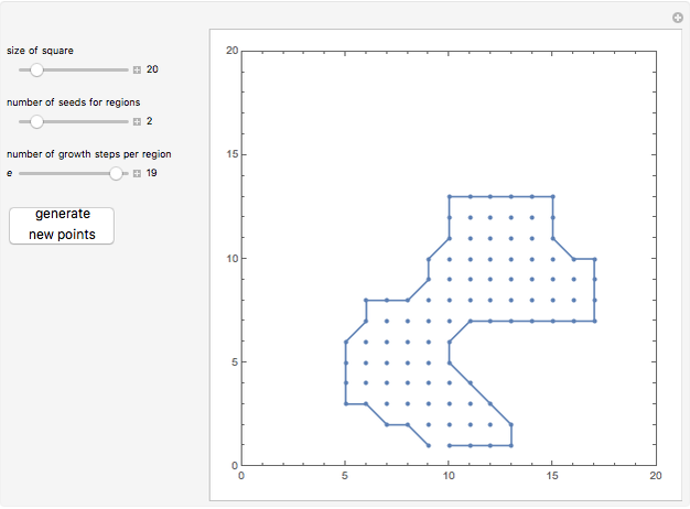
In the Demonstration, choose settings and generate points to see how the different components are identified and boundaries drawn. You can also notice that if the seeds are closely located, with adequate expansions, the components coalesce, yielding a single boundary.
References
[1] Wikipedia. "Connected-Component Labeling." (Jan 27, 2015) en.wikipedia.org/wiki/Connected-component_labeling.
[2] Wikipedia. "Moore Neighborhood." (Jan 27, 2015) en.wikipedia.org/wiki/Moore_neighborhood.
Permanent Citation
 Boundary and Hole Detection
Raja Kountanya B-Spline Curve with Boundary Conditions
M. Szilvási-Nagy Ray Tracing for Points in a Polygon
Raja Kountanya Elementary Cellular Automaton Process Visualization
Michael Schreiber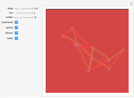 Constrained Optimal Routes in 3D Space
Vitaliy Kaurov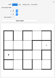 Mazes on Various Surfaces
Izidor Hafner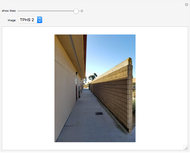 Finding the Vanishing Points of Sample Images
Simon Kim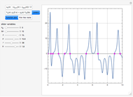 A Graphically Enhanced Method for Computing Real Roots of Nonlinear Functions
Housam Binous and Brian G. Higgins The Homicidal Chauffeur Problem
Aaron T. Becker and Javier Garcia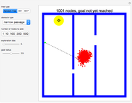 Rapidly Exploring Random Tree (RRT) and RRT*
Aaron T. Becker and Li Huang
-
 Yield under a Rigid Toroidal Indenter
Raja Kountanya -
 Shear-Angle Models for Oblique Metal Cutting
Raja Kountanya -
Ray Tracing for Points in a Polygon
Raja Kountanya -
Boundary and Hole Detection
Raja Kountanya -
 Component Identification and Boundary Delineation
Raja Kountanya -
 Using Eigenvalue Analysis to Rotate in 3D
Raja Kountanya -
 Chatter Stability with Orthogonal Rotation
Raja Kountanya -
 Boundary Value Problems for Cone Geodesics
Raja Kountanya