Finite Potential Well


Requires a Wolfram Notebook System
Interact on desktop, mobile and cloud with the free Wolfram Player or other Wolfram Language products.
This Demonstration illustrates the solutions of the transcendental equations that arise in solving for the bound-state energies and eigenfunctions of a quantum-mechanical particle interacting with a one-dimensional finite square-well potential. It also qualitatively shows how these solutions satisfy the boundary conditions required of bound-state eigenfunctions.
Contributed by: Michael R. Braunstein (Central Washington University) (March 2011)
Open content licensed under CC BY-NC-SA
Snapshots


Details
In this Demonstration, solutions of the transcendental equation for the quantum mechanical bound-state energies,  , and eigenfunctions,
  , are shown for a particle in a finite one-dimensional square well. The parameters of the system are the width of the square well,
  , its depth,
  , and the mass of the particle,
  . The solutions of this system are conveniently expressed in terms of the dimensionless parameters
  and
and  . We can think of
  as the "strength of the interaction" between the particle and the well, and note that
  is related to the ratio of the energy of the particle to the depth of the well.
The solutions are obtained in the typical manner for a discontinuous potential: functions satisfying the time-independent Schrödinger wave equation are found for each region of the potential, and then boundary conditions are applied: the symmetry of the potential requires that the eigenfunctions be either symmetric or antisymmetric with respect to the origin, the eigenfunctions must be normalizable, and because the discontinuities in the potential are finite, the eigenfunctions and their first derivatives must be continuous at the boundaries between regions.
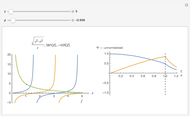
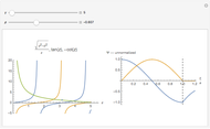
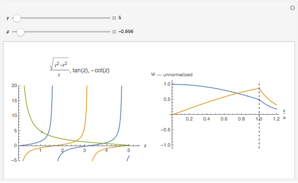
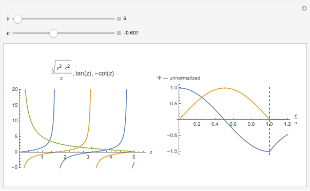
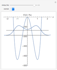
Applying this approach, we find that the eigenfunctions are sinusoidal in the well, exponentially decreasing outside the well, and that transcendental equations express the conditions that satisfy the boundary requirements between regions: for the symmetric eigenfunctions, and for the antisymmetric eigenfunctions. In the left-hand plot, as a function of is represented by the gold line, as a function of by the blue lines, and as function of by the red lines.
For a particular value of (remember, this can be thought of as the "strength of the interaction" between the particle and the well), where the gold line intersects the blue lines corresponds to eigenfunctions and energies that satisfy the boundary conditions for symmetric eigenfunctions, and where the gold line intersects the red lines corresponds to eigenfunctions and energies that satisfy the boundary conditions for antisymmetric eigenfunctions.
As you adjust the ratio (the ratio of the bound-state energy to the depth of the well—its value is negative to indicate a bound state), a corresponding dot moves along and when it is located at one of the intersections, the value of corresponds to an allowed bound-state energy of the system!
The right-hand plot shows the unnormalized eigenfunctions as a function of position (symmetric: blue; antisymmetric: red) in the region between the origin and one of the boundaries of the potential well (represented with a dashed vertical line). Adjust the ratio to see that generally the sinusoid inside the well and the exponential outside the well have different slopes at the boundary, showing that they do not satisfy the boundary conditions, BUT the slopes match when the condition is met for the symmetric eigenfunctions and is met for the anti-symmetric eigenfunctions!
Some other important things to note are that increasing (the "strength of the interaction") increases the number of bound states available to the system, and that the number of antinodes of an eigenfunction is qualitatively related to its energy.
For more information about this system see, for instance, section 2.6 and problem 2.29 of D. J. Griffiths, Introduction to Quantum Mechanics, 2nd ed., Upper Saddle River, NJ: Pearson/Prentice Hall, 2005.
Permanent Citation
"Finite Potential Well"
http://demonstrations.wolfram.com/FinitePotentialWell/
Wolfram Demonstrations Project
Published: March 7 2011
 Numerov Solutions for Single- and Double-Well Potentials
Eric R. Bittner Time-Evolution of a Wavepacket in a Square Well
Michael Trott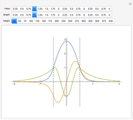 Energy Spectrum for a Finite Potential Well
Adam Strzebonski Scattering by a Square-Well Potential
M. Hanson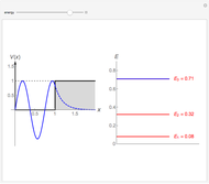 Boundary Conditions for a Semi-Infinite Potential Well
Porscha McRobbie and Eitan Geva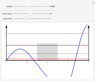 Perturbed Infinite Square Well
Martha Takats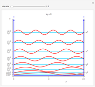 Exact Numerical Solutions for the Stepped-Infinite-Square Well
M. Hanson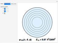 Particle in an Infinite Spherical Well
S. M. Blinder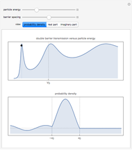 Double Delta Function Scattering Potential
Peter Falloon Variational Method Applied to Stepped-Infinite-Square-Well Energies
M. Hanson