Fish-in-Pond Simulation

Requires a Wolfram Notebook System
Interact on desktop, mobile and cloud with the free Wolfram Player or other Wolfram Language products.
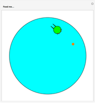
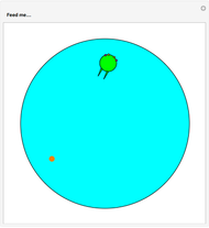
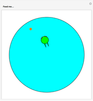
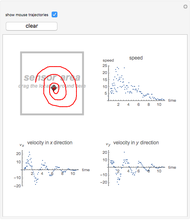
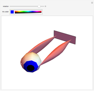
A fish is swimming in a circular pond as shown. It uses its sensory organs to detect both food in the pond and the hazard (the pond edge) in order to generate the correct response, swimming toward the food but away from the pond edge. See the Details section to learn about mechanical and sensory modelling.
[more]
Contributed by: Te-yuan Chyou (March 2011)
Suggested by: Mike Paulin
Open content licensed under CC BY-NC-SA
Snapshots


Details
1. Equation of motion
Assume that the fish body is spherical, and the position and the orientation of the fish in 2D can be described in generalized coordinates  . The equations of motion of the fish can be written as
 ,
,
 ,
,
 ,
,
 ,
,
where  is the mass of the fish,
  is the radius, and
  and
and  are damping coefficients due to the viscosity of water.
  and
and  are control forces, generated from the left and right fins in response to any signals received from the eyes and ears. The angle
  is constant, which is the angle between the axis of symmetry and the line joining the center of the spherical body and the fin bases. The coefficients
  and
and  are arbitrary constants.
Assume that the fish is small and light, and the inertial force term is negligible; the equation of motion becomes
 ,
,
 .
.
Hence the equations of motion under the assumption of small mass and size takes the form
 ,
,
 ,
,
 .
.
2. Sensory modelling
2.1 Weber–Fechner Law
Electrophysiology (recording neurons with electrodes) and psychophysics (asking people or testing animals to discover what they perceive) show that we register constant relative changes in stimulus intensity as constant changes. This means that we can model the response of a sense organ as a logarithmic function of the stimulus intensity:
 ,
,
where  is stimulus intensity and
  is the response amplitude.
2.2 Wall sensor
When the fish moves in water it displaces water ahead and around it. This water that gets pushed aside is called the bow wave. A solid object in the bow wave causes a change in the flow pattern over the fish’s skin as it swims by. This is called the acoustic near-field effect. The intensity of an acoustic near-field pattern falls exponentially with distance to the source. Applying the Weber–Fechner Law, the response due to the wall sensor (ear) stimulus can be written as
 .
.
2.3 Prey sensor
We will assume that the prey or food generates some cue (e.g. light or sound or smell) that decreases following the inverse-square law as the fish moves away from it. The inverse-square law is a physically correct model of light, sound, or smell from a localized source under idealized conditions. Again, applying the Weber–Fechner Law, the response due to the prey/food sensor (eyes) stimulus can be written as
 .
.
The parameter  is infinitesimal; it is included as the conventional inverse-square law may result in a divide-by-zero exception and crash the program.
2.4 Force due to stimuli  and )
and )
The magnitude of the force generated in each fin is proportional to the strength of the responses. The fish has two eyes and ears, so it can determine whether the wall or the prey is on the right or left, as by geometry one of the eyes or ears will receive a stronger stimulus.
We want the fish to rotate away from the wall, but also rotate toward the food. If (for example), there is a wall on the left, then the left ear receives a stronger signal than the right ear. We want to push with the left fin to make the fish turn right, away from the wall, so we want to increase the force on the left fin while reducing the force on the right.
Therefore, and can be calculated using
 ,
,
where  and
and  are the forces generated by the fins when there are no stimuli.
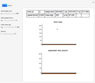
3. Simulation
In the simulation, we discretize the equation of motion and introduce a stochastic term  to model the noise.
 ,
,
 ,
,
 .
.
Permanent Citation
 Moon Landing Simulation
Valeriu Ungureanu and Alexandru Brega Simulation of Feedback Control System with Controller and Second-Order Plant
Nasser M. Abbasi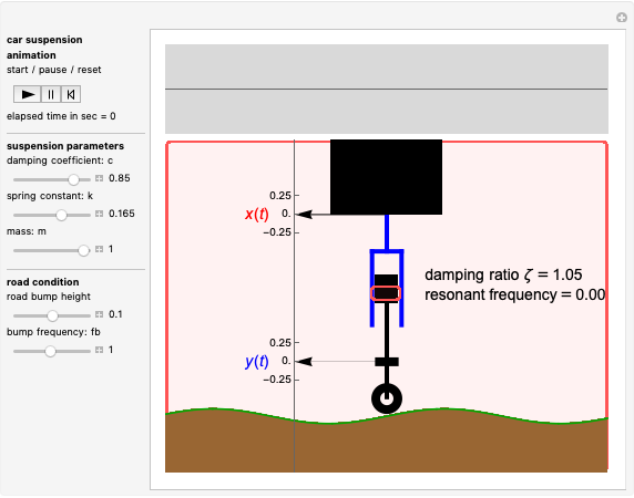 Simulating Vehicle Suspension with a Simplified Quarter-Car Model
Erik Mahieu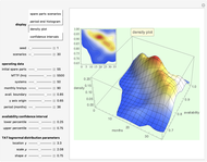 System Availability
Michail Bozoudis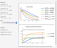 System Reliability
Michail Bozoudis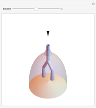 Lung Model Simulation
Enrique Zeleny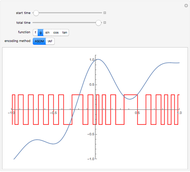 Time Encoding of Analog Signals
Andre Kessler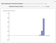 Hopfield Network with State-Dependent Threshold
Vaibhav Vavilala and Yogesh Joglekar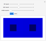 The Simultaneous Contrast Effect
Rob Morris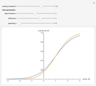 Comparing the Normal Ogive and Logistic Item Characteristic Curves
Vincent Kieftenbeld
-
 Fish-in-Pond Simulation
Te-yuan Chyou -
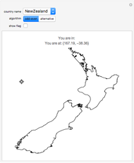 Country Interior: Two Solutions to the Nonconvex Polygon Interior Problem
Te-yuan Chyou -
 The Block Pushing Game
Te-yuan Chyou -
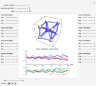 Dynamics of a Cube-Shaped Mass-Spring Network
Te-yuan Chyou -
 Building a Velocity Sensor
Te-yuan Chyou -
 Eyeball and Two Muscles
Te-yuan Chyou -
 Inside World of the Torus
Te-yuan Chyou -
 Rimless Wheel Locomotion
Te-yuan Chyou