Numerical Approximation of the Fourier Transform by the Fast Fourier Transform (FFT) Algorithm


Requires a Wolfram Notebook System
Interact on desktop, mobile and cloud with the free Wolfram Player or other Wolfram Language products.
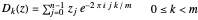
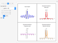
The Fourier transforms of some classical functions are calculated and their real and imaginary parts are plotted. The Fourier transform (FT) is numerically calculated by using the step function approximation to the Fourier integral; this finally leads to the discrete Fourier transform (DFT).
[more]
Contributed by: Blazej Radzimirski (March 2011)
Open content licensed under CC BY-NC-SA
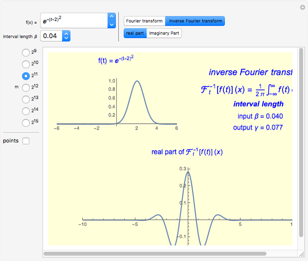
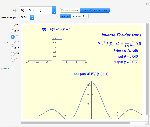
Snapshots

Details
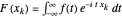
The continuous Fourier transform (CFT) of a function  and its inverse are defined by
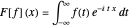 InlineMathColumns=,Columns
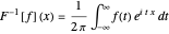 InlineMathColumns=.Columns
A numerical approximation of the CFT requires evaluating a large number of integrals, each with a different integrand, since the values of this integral for a large range of  are needed.
The FFT can be effectively applied to this problem as follows. Let us assume that  is zero outside the interval
  . Let
. Let  be the sample spacing in
  for the
  input values of
  , which are assumed to be centered at zero, where
  is even. The values of
  and
and  are chosen at the beginning in this procedure so the range of the interval
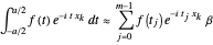
  is changing and depends on these parameters. The abscissas for the input data are
  ,
,  . Then we can write
 InlineMathColumns
 =InlineMathColumns=Columns
 =InlineMathColumns=Columns
 =InlineMathColumns=Columns
 =InlineMathColumns=.Columns
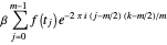
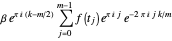
We define  ,
,  . This is necessary for the above expression to be in the form of the DFT, denoted here by
  :
:
 ..InlineMathColumns
The sample spacing (i.e., the resolution) of the result is fixed at the value  as soon as one specifies the number
  of sample points and their interval
  . The above definition of the DFT is equivalent to the Mathematica command Fourier[list, FourierParameters->{1,-1}].
Usually, comparable sample spacing intervals in  and
and  are required. Then, one must put
  , or
, or  . It is clear that if one wishes to obtain accurate, high-resolution results using this procedure, then it may be necessary to set
  very large.
More details can be found in D. H. Bailey and P. N. Swarztrauber, "A Fast Method for the Numerical Evaluation of Continuous Fourier and Laplace Transform," SIAM Journal on Scientific Computing, 15(5), 1994 pp. 1105–1110.
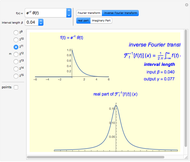
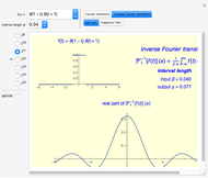
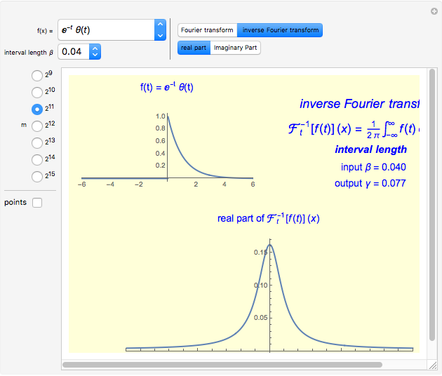
You can choose the number of data points  (an integer power of two) from the radio button menu. The appropriate value of the output sample interval
  for a given
  is displayed after choosing the input sample spacing
  . To show the sample points in the initial function (every fourth sample point is showed) and that the CFT in this algorithm is obtained in the form of points, check "points".
It is very convincing to fix a sample spacing  from the popup menu and decrease the number of sampling points
  : you can then observe the deterioration of the accuracy of the Fourier transform.
Permanent Citation
 XFT: An Improved Fast Fourier Transform
Rafael G. Campos, J. Jesus Rico Melgoza, and Edgar Chavez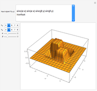 XFT2D: A 2D Fast Fourier Transform
Rafael G. Campos, J. Jesus Rico Melgoza, and Edgar Chavez Fourier Transform Pairs
Porscha McRobbie and Eitan Geva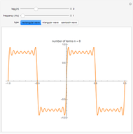 Approximation of Discontinuous Functions by Fourier Series
David von Seggern (University Nevada-Reno)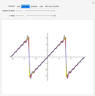 Fourier Series of Simple Functions
Alain Goriely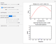 Fourier Power Spectrum as a Measure of Line Jaggedness
Mark D. Normand and Micha Peleg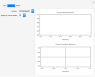 Comparing Fourier Series and Fourier Transform
Martin Jungwith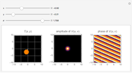 Amplitude and Phase in 2D Fourier Transforms
Katherine Rosenfeld Numerical Inversion of the Laplace Transform: The Fourier Series Approximation
Housam Binous Orthogonality of Two Functions with Weighted Inner Products
Alain Goriely