Quantum Harmonic Oscillator Tunneling into Classically Forbidden Regions


Requires a Wolfram Notebook System
Interact on desktop, mobile and cloud with the free Wolfram Player or other Wolfram Language products.
This Demonstration shows coordinate-space probability distributions for quantized energy states of the harmonic oscillator, scaled such that the classical turning points are always at  .
.
Contributed by: Arkadiusz Jadczyk (January 2015)
Open content licensed under CC BY-NC-SA
Snapshots


Details
Think about a classical oscillator, a swing, a weight on a spring, a pendulum in a clock…. They have a certain characteristic spring constant and a mass. For simplicity, choose units so that these constants are both 1. Also assume that the time scale is chosen so that the period is  . Given energy
  , the classical oscillator vibrates with an amplitude
  . Its deviation
  from the equilibrium position
  is given by the formula
 .
.
The relationship between energy and amplitude is simple:  . For a classical oscillator, the energy can be any positive number.
For a quantum oscillator, assuming units in which Planck's constant  , the possible values of energy are no longer a continuum but are quantized with the possible values:
  . To each energy level there corresponds a quantum eigenstate; the wavefunction is given by
 ,
,
where  is a Hermite polynomial. This wavefunction (notice that it is real valued) is normalized so that its square
  gives the probability density of finding the oscillating point (with energy
  ) at the point
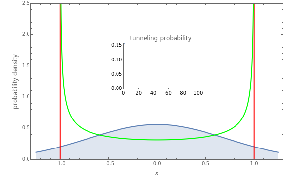
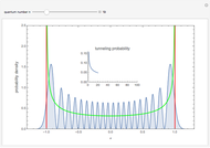
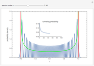
  . Classically, there is zero probability for the particle to penetrate beyond the turning points
  and
and  . But for the quantum oscillator, there is always a nonzero probability of finding the point in a classically forbidden region; in other words, there is a nonzero tunneling probability.
One popular quantum-mechanics textbook [3] reads: "The probability of being found in classically forbidden regions decreases quickly with increasing  , and vanishes entirely as approaches infinity, as we would expect from the correspondence principle."
This Demonstration calculates these tunneling probabilities for  . The calculation is done symbolically to minimize numerical errors.
You can see the sequence of plots of probability densities, the classical limits, and the tunneling probability for each . There is also a U-shaped curve representing the classical probability density of finding the swing at a given position given only its energy, independent of phase. Each graph is scaled so that the classical turning points are always at  and
and  . The vertical axis is also scaled so that the total probability (the area under the probability densities) equals 1.
It can be seen that indeed, the tunneling probability, at first, decreases rather rapidly, but then its rate of decrease slows down at higher quantum numbers . While the tails beyond the red lines (at the classical turning points) are getting shorter, their height is increasing.
References
[1] J. L. Powell and B. Crasemann, Quantum Mechanics, Reading, MA: Addison-Wesley, 1961 p. 136.
[2] B. Thaller, Visual Quantum Mechanics: Selected Topics with Computer-Generated Animations of Quantum-Mechanical Phenomena, New York: Springer, 2000 p. 168.
[3] P. W. Atkins, J. de Paula, and R. S. Friedman, Quanta, Matter and Change: A Molecular Approach to Physical Chemistry, New York: Oxford University Press, 2009 p. 66.
Permanent Citation
 Time Evolution of Squeezed Quantum States of the Harmonic Oscillator
Arkadiusz Jadczyk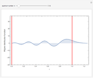 Wigner Distribution Function for Harmonic Oscillator
Arkadiusz Jadczyk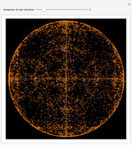 Quantum Octahedral Fractal via Random Spin-State Jumps
Arkadiusz Jadczyk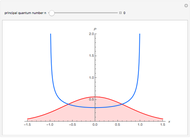 Quantum/Classical Correspondence for the Harmonic Oscillator
Niels Walet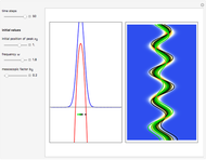 Continuous Transition between Quantum and Classical Behavior for a Harmonic Oscillator
Partha Ghose and Klaus von Bloh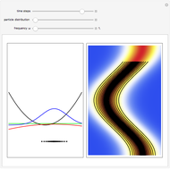 Causal Interpretation of the Quantum Harmonic Oscillator
Klaus von Bloh Coupled Quantum Harmonic Oscillators
Humberto Munoz Bauza Superposition of Quantum Harmonic Oscillator Eigenstates: Expectation Values and Uncertainties
Porscha McRobbie and Eitan Geva Eigenstates of the Quantum Harmonic Oscillator Using Spectral Methods
Housam Binous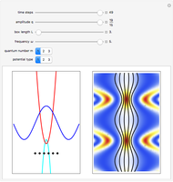 The Quantum Harmonic Oscillator with Time-Dependent Boundary Condition in the Causal Interpretation
Klaus von Bloh
-
 Dzhanibekov Effect
Arkadiusz Jadczyk -
Time Evolution of Squeezed Quantum States of the Harmonic Oscillator
Arkadiusz Jadczyk -
Quantum Octahedral Fractal via Random Spin-State Jumps
Arkadiusz Jadczyk -
Wigner Distribution Function for Harmonic Oscillator
Arkadiusz Jadczyk -
 Quantum Harmonic Oscillator Tunneling into Classically Forbidden Regions
Arkadiusz Jadczyk