Records in Sequences of Random Variables


Requires a Wolfram Notebook System
Interact on desktop, mobile and cloud with the free Wolfram Player or other Wolfram Language products.
Consider a sequence of real numbers  ,
,  , …. A value
  is a record value (or a high-water mark) if it is the largest value among all the values that have been recorded up to time
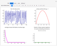
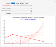
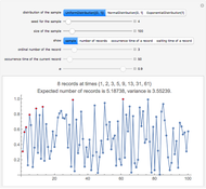
  ; is always a record. This Demonstration shows a sample for one of three distributions and its records with a red color. The Demonstration also shows the distribution of the number of records for samples of sizes 10, 20, …, 1000; the distribution of the occurrence time of the
  record,
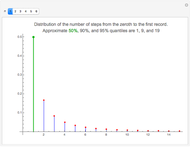
  ; and the conditional upper bounds of waiting times for the next record.
Contributed by: Heikki Ruskeepää (October 2013)
Open content licensed under CC BY-NC-SA
Snapshots


Details
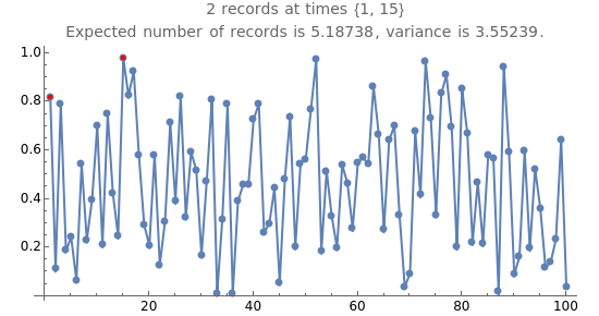
Snapshot 1: Among the 100 observations from a uniform distribution, there happen to be 8 records; the expected number of records for a series of 100 values is 5.2.
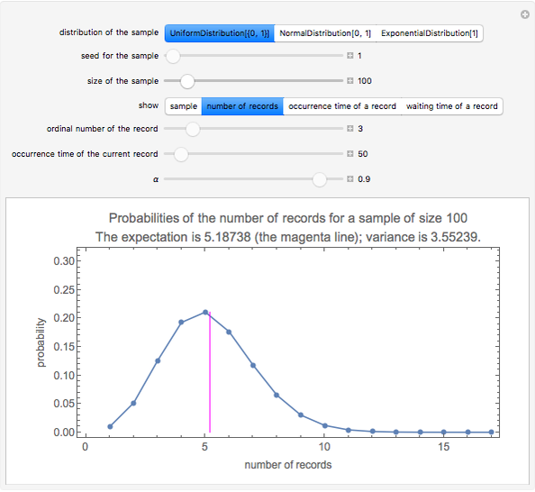
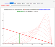
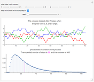
Snapshot 2: Here are the probabilities that there are 1, 2, …, 17 records in a series of 100 values. The magenta line is at the expectation 5.2. There is a very small probability that there are more than, say, 10 records among 100 values. Theoretically, there could be as few as one record (it has approximately a probability of 0.01) and as many as 100 records (which must have a very tiny probability). The Demonstration only shows the probabilities up to the  record.
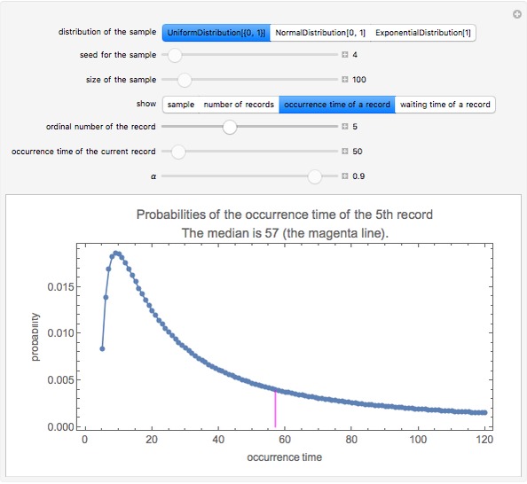
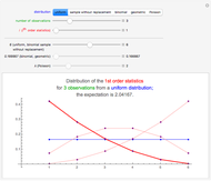
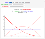
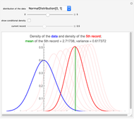
Snapshot 3: This plot shows the probabilities of the occurrence times of the fifth record. The earliest occurrence time is 5 (it has a probability of approximately 0.008). The most probable occurrence time is 9 (with a probability of approximately 0.019). The median is 57 (the mean is infinite). Thus, with several sequences, in approximately half of them the fifth record is among the first 57 values; in another half of the sequences, the fifth record occurs later. There is no upper bound for the occurrence time of the fifth record; it could be, say, larger than 1000. The Demonstration only shows the probabilities of some small values of the occurrence time.
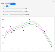
Snapshot 4: The plot shows conditional upper bounds for the waiting times of records. In the first snapshot, the seventh record occurred at time 31. Given that the occurrence time of a record is 31, the plot shows that the next record is among the next 279 values with probability 0.9; with probability 0.1, more values are needed to get the next record (from the first snapshot, the next record (the eighth) was actually the  value after the seventh record).
Expected Number of Records
Let , …,  be independent, identically distributed continuous random variables. Let
  be the total number of records in the sequence , …, . The expected value of is
  , that is,
  is the
  harmonic number. For example, for sequences of length 10, 100, 1000, 10000, 100000, or 1000000 the expected number of records is 2.9, 5.2, 7.5, 9.8, 12.1, and 14.4, respectively. The lengths of the sequence needed so that the expected number of records for the first time is at least 2, 3, …, 10 are 4, 11, 31, 83, 227, 616, 1674, 4550, and 12367, respectively. For example, for the mean number of records to be 10, we need a sequence of 12,367 values, which is the number of terms in the harmonic series required to make the sum exceed 10. Near the beginning of the sequence, records occur quite frequently, but after that, new records occur increasingly seldom. Thus, except initially, records are seldom.
As a practical example [1, p. 65], assume that the maximum yearly temperatures in a given city can be considered to be values of approximately independent, identically distributed random variables. A person at the ages 4, 11, 31, or 83 years has seen 2, 3, 4, and 5 temperature records on average, respectively.
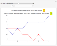
As another example [1, p. 78], to find the weakest board among 100 boards, stress the first board to its failure point. Stop the test of the second board if it survives the stress applied to the first board. By continuing similarly with the rest of the boards, the expected number of broken boards is only 5.2.
Distribution of the Number of Records
Let  be the probability that in a series of length
  there will be exactly
  records. Rényi showed that
  where
where  and
and  is a Stirling number of the first kind. For example, in a sequence of length 6, the probabilities that there will be 1, 2, 3, 4, 5, or 6 records are 0.1667, 0.3806, 0.3125, 0.1181, 0.0208, and 0.0014, respectively.
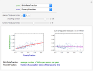
Occurrence Time of a Record
Let  be the time at which we have the record (
 ). It can be shown that
  ,
,  , where
  is as before. The expected value of is infinite for
  . This Demonstration shows the median of the distribution of . The medians for = 2, 3, …, 10, are 2, 7, 21, 57, 157, 430, 1173, 3199, and 8717, respectively. For example, consider a large number of independent sequences; in about half of them the fifth record occurs no later than at time 57 and in the other half of them the fifth record occurs later than at time 57.
Waiting Time to the Next Record
Let  be the interrecord waiting time, that is, the time elapsed between the and the
  records. The conditional distribution of
  , conditioned on , is
  . An
. An  such that this probability is a given value
  is
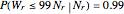
is  . For example, if is 0.5, 0.9, 0.95, or 0.99, then is ,
  ,
,  , and
, and  , respectively. This means that
 ,
,
 ,
,
 ,
,
 .
.
For example, if the current record (the record) occurred at time , then with probability 0.5 the next record is among the next values; with probability 0.5, more values are needed to get the next record. Similarly, with probability 0.9, the next record is among the next values.
As a numerical example, let the fifth record occur at time 50:  . Then
 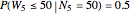 , that is, the sixth record with probability 0.5 is among the next 50 values; with probability 0.5, we have to wait longer. As another example, is 450 so that
 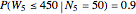 , that is, the sixth record with probability 0.9 is among the next 450 values.
A Note
Not one of the results mentioned here depends on the actual distribution of the variables ; we only need the assumption that these variables are independent, identically distributed, continuous random variables. In this Demonstration, the choices between uniform, normal, and exponential variables are offered only to show that, for each distribution, the samples have similar properties for records.
The Demonstration is based on [1, pp. 63–78].
Reference
[1] J. Andel, Mathematics of Chance, New York: Wiley, 2001.
Permanent Citation
 Distribution of Discrete Records
Heikki Ruskeepää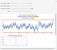 A Reluctant Random Walk
Heikki Ruskeepää Polynomial Fits of Random Walks
Michael Schreiber Hypothesis Tests about a Population Mean
Chris Boucher The Power of a Test Concerning the Mean of a Normal Population
Chris Boucher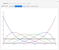 Distributions of Order Statistics
Chris Boucher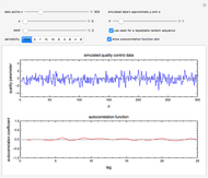 Hidden Periodicity in Quality Control Records
Mark D. Normand and Micha Peleg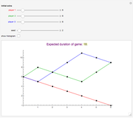 A Curious Coin-Flipping Game
Heikki Ruskeepää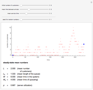 Simulating the M/M/1 Queue
Heikki Ruskeepää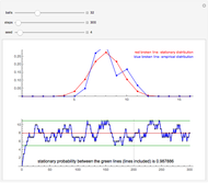 Simulating the Bernoulli-Laplace Model of Diffusion
Heikki Ruskeepää
-
 Obtuse Random Triangles from Three Points in a Rectangle
Heikki Ruskeepää -
 Chaotic Data: Maximal Lyapunov Exponent
Heikki Ruskeepää -
 Chaotic Data: Correlation Dimension
Heikki Ruskeepää -
 Chaotic Data: Delay Time and Embedding Dimension
Heikki Ruskeepää -
 Method of Support Vector Regression
Heikki Ruskeepää -
 Local Regression for Country Data
Heikki Ruskeepää -
 Distribution of the Sample Range of Continuous Random Variables
Heikki Ruskeepää -
 Distribution of the Sample Range of Discrete Random Variables
Heikki Ruskeepää -
 Distributions of Discrete Order Statistics
Heikki Ruskeepää -
 Distributions of Continuous Order Statistics
Heikki Ruskeepää -
 Waiting for the Next Record
Heikki Ruskeepää -
Distribution of Discrete Records
Heikki Ruskeepää -
 Records in Sequences of Random Variables
Heikki Ruskeepää -
 Distribution of Records
Heikki Ruskeepää -
 The Three-Tower Problem
Heikki Ruskeepää -
 Walking Randomly Until No Shoes Are Available
Heikki Ruskeepää -
A Reluctant Random Walk
Heikki Ruskeepää -
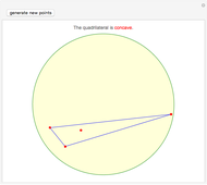 Concave Random Quadrilaterals from Four Points in a Disk
Heikki Ruskeepää -
 Obtuse Random Triangles from Three Parts of the Unit Interval
Heikki Ruskeepää -
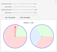 Spin Game
Heikki Ruskeepää