Best Response Learning in a Cournot Framework


Requires a Wolfram Notebook System
Interact on desktop, mobile and cloud with the free Wolfram Player or other Wolfram Language products.
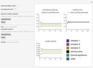
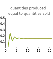
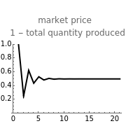
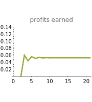
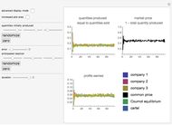
This Demonstration shows how three companies can interact within a Cournot competition with noise and beliefs. It shows the effect of different beliefs regarding the reaction of the competitors and noise in the market. To illustrate this, the individual production levels, the individual profits, and the price level are plotted with respect to time. The interaction of the companies is modelled through a best response learning process.
Contributed by: Clemens Fiedler (September 2013)
Open content licensed under CC BY-NC-SA
Snapshots


Details
Within the Cournot model of competition, a number of companies (three in this Demonstration) compete via producing a homogeneous good. The price is set through a process of supply and demand after each company has decided their production quantity. In this model, the demand function is assumed to be equal to  , where
  is the total quantity produced by all of the companies. Thus, the revenue of company
  is
is  , where
  denotes the production of company .
Each company incurs costs based on their production. The costs for company are assumed to be quadratic:  ; thus, marginal costs are increasing. The profits of company are consequently defined as
 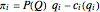 .
.
Taking the first derivative with respect to yields a reaction function, the optimal (profit maximizing) quantity for a company given a fixed production level of its competitors.
The production decision of each company is based on the production level of each competitor in the last period. Thus, the companies react based on their production levels. This process converges to the Cournot equilibrium (given the parameters assumed).
Use the "anticipated reaction" sliders to define each company's belief about the reaction of its competitors. For example, if this parameter is  for company 1, then the first company believes that an increase of its quantities by 1 unit will lead to an increase of both other companies production by . In general, a value of
  implies that the company assumes aggressive competitors, whereas
  implies defensive competitors. Such a model is referred to as conjectural variation.
Additionally, you can set a random error term, such that the amount produced by each company deviates by a certain amount from their choice.
The effect of the initial quantities on the model development is practically nil and vanishes after a small number of steps.
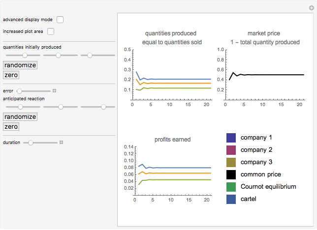
The parameter of conjectural variation does not adversely affect the convergence to the equilibrium; it does, however, affect the amounts produced in the equilibrium. Overly optimistic companies with a belief in defensive adversaries produce a larger amount of goods and achieve higher profits (see Snapshot 1).
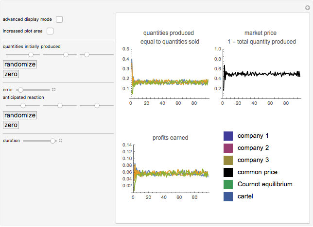
The error term will only increase the region of convergence and not the equilibrium. The amounts produced, and thus profits and the price, will still converge to a region around the equilibrium (see Snapshot 2).
However, if the parameter of conjectural variation is in stark contrast to reality, the equilibrium might no longer exist. For example, if company 1 and company 2 both assume defensive competitors, both will increase their production, thus violating their assumptions. Since the prices are then too low, they will decrease their production, thus increasing prices. As both companies are not able to learn from this, they will again increase their production, thus causing a second crash of the price (see Snapshot 3).
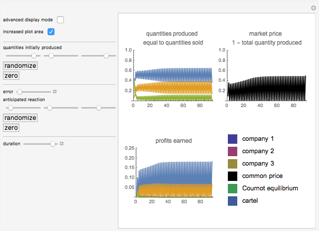
Interestingly, if all three companies have large positive parameters of conjectural variation, the result yields prices near the prices set by a cartel (see Snapshot 4).
Permanent Citation
 Cournot Competition with Two Firms
Kazuki Kumashiro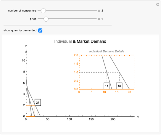 Individual versus Market Demand
Samuel G. Chen Customer Profitability with the Whale Curve
Thomas Laussermair Profit Maximization in Perfect Competition
Fiona Maclachlan Property Coinsurance
Seth J. Chandler Spotting a Liquidity Trap
Samuel G. Chen Money Creation in the Banking System
Alla Ahmad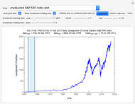 Fate of a Long-Term Index Fund Investment According to the S&P 500
Mark D. Normand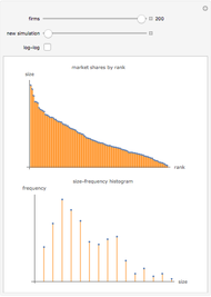 A Model of Market Shares II
Fiona Maclachlan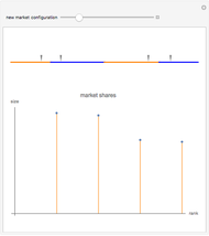 A Model of Market Shares I
Fiona Maclachlan