Brownian Motion in 2D and the Fokker-Planck Equation

Requires a Wolfram Notebook System
Interact on desktop, mobile and cloud with the free Wolfram Player or other Wolfram Language products.
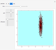
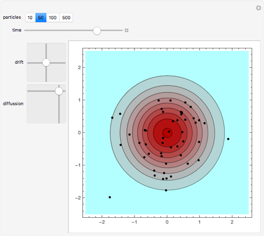
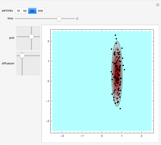
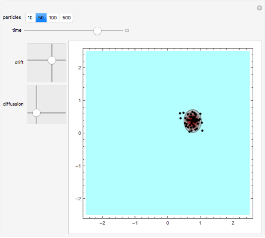
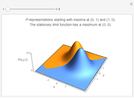
We show the Brownian motion of an evolving assembly of particles and the corresponding probability density. The probability density is a solution of the Fokker–Planck equation, which here reduces to a drift-diffusion partial differential equation. The center of mass of the particle distribution moves with a constant drift velocity while anisotropic diffusion is determined by the principal values of the diffusion matrix, along the Cartesian axes.
Contributed by: Alejandro Luque Estepa (March 2011)
Open content licensed under CC BY-NC-SA
Snapshots


Details
Brownian motion of a particle is described by a stochastic differential equation  , where the
  are particle positions in
  ,
,  is the drift velocity,
  is an
is an  matrix and
  represents an
  -dimensional normal Wiener process. The Fokker–Planck equation (also called forward Kolmogorov equation) describes the temporal evolution of the probability density
  :
:
 , where
  .
.
If and  are constant, the Fokker–Planck equation reduces to a drift-diffusion equation that can be solved analytically. The fundamental solutions are Gaussian distributions which drift and widen with time.
This Demonstration shows the Brownian motion of a number of independent particles in 2D superimposed on the solution of the Fokker–Planck equation. To simplify the controls, the principal axes of the matrix are always the horizontal-vertical axes of the screen.
Permanent Citation
 Shape-Invariant Solutions of the Quantum Fokker-Planck Equation for an Optical Oscillator
Reinhard Tiebel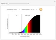 Blackbody Spectrum
Jeff Bryant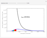 Blackbody Radiation
Zach Heuman (Boise State University)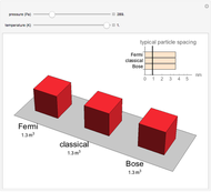 Compressing Ideal Fermi and Bose Gases at Low Temperatures
Tad Hogg Boltzmann Gas
Gianni Di Domenico (Université de Neuchâtel) and Antoine Weis (Université de Fribourg) Classical Correlation Function via Generalized Langevin Equation
Yifan Lai Approach of a System of Particles towards Thermal Equilibrium
Ulrich Mutze and Stephan Leibbrandt Statistical Behavior of a Set of Uniformly Rotating Independent Particles with Random Frequencies
Martina Luigi Comparing Properties of Chemical Elements
Stephen Wolfram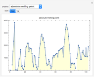 Properties of Chemical Elements
Stephen Wolfram
-
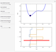 Logical Stochastic Resonance
Alejandro Luque Estepa -
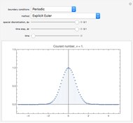 Numerical Solution of the Advection Partial Differential Equation: Finite Differences, Fixed Step Methods
Alejandro Luque Estepa -
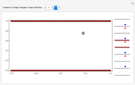 Method of Image Charges: Point Charge inside a Planar Capacitor
Alejandro Luque Estepa -
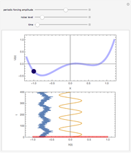 Stochastic Resonance
Alejandro Luque Estepa -
 Brownian Motion in 2D and the Fokker-Planck Equation
Alejandro Luque Estepa