Fractal Curves Generated by Fourier Series

Requires a Wolfram Notebook System
Interact on desktop, mobile and cloud with the free Wolfram Player or other Wolfram Language products.
Given a sequence of coefficients  ,
,  , write the Fourier series
 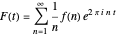 . For
. For  , the plot of
  traces out a closed curve in the complex plane. This Demonstration shows this curve for some selected choices of the coefficients
  .
.
Contributed by: Nick Kokkines, Andre Park, Efstathios Konstantinos Chrontsios Garitsis and A. J. Hildebrand (August 2022)
(Based on an undergraduate research project at the Illinois Geometry Lab in Fall 2021)
Open content licensed under CC BY-NC-SA
Snapshots
Details
This Demonstration is inspired by a 1995 paper by J. Bohman and C.-E. Fröberg [1] investigating the Fourier series
for various classes of oscillating coefficients  . In many cases, they observed remarkable fractal-like patterns in the plots of
  . More recent work by E. Kowalski and W. F. Sawin [2] examines the behavior of series of this type from a probabilistic point of view. Their work sheds some light on the peculiar shape of the curve traced out by
  when the coefficients
  are given by the Möbius function.
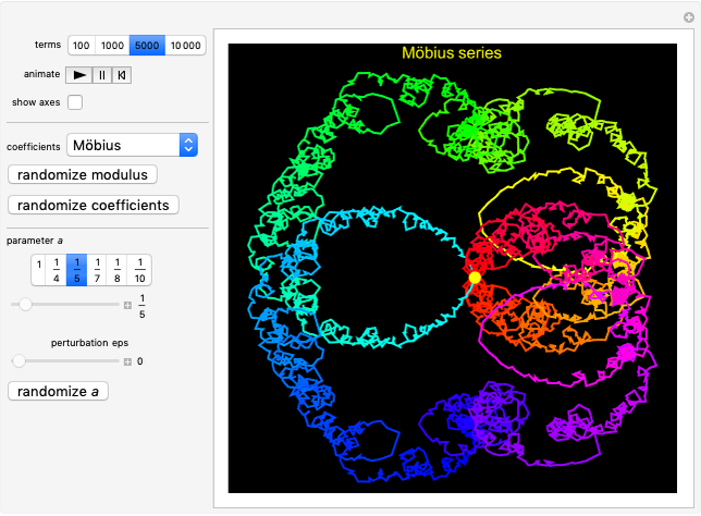
This Demonstration shows the closed curve in the complex plane traced out by  as
as  ranges from 0 to 1 for the following coefficient sequences
  :
:
Möbius:  , where
  is the Möbius function.
Jacobi symbol:  , where the modulus
  is a prime in the range
  , selected randomly. Use the "randomize modulus" button to generate a new randomization.
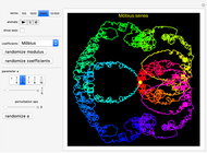
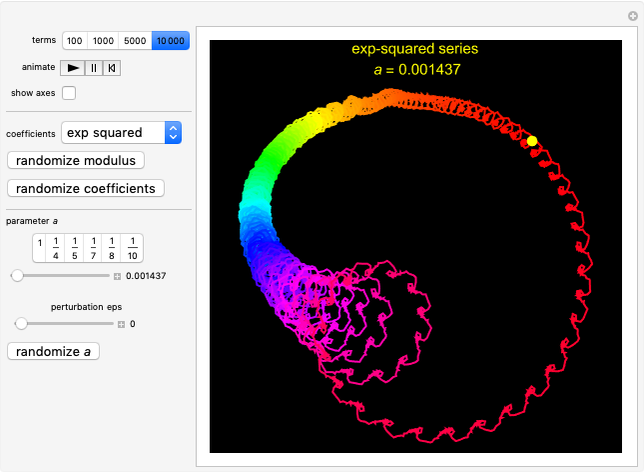
Exp-squared:  , in which you set the parameter
  in the range
  . Of particular interest is the behavior of the associated Fourier series
  in the case when the parameter
  is close to a rational number with a small denominator. To study this behavior, this Demonstration offers a list of predefined rational values for
  . Use the "perturbation" slider to perturb the parameter
  over a narrow range.
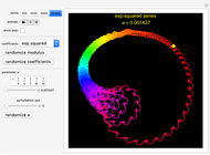
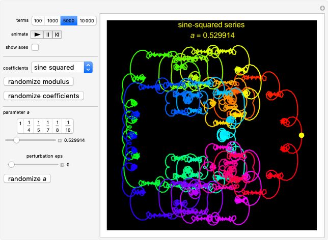
Sine-squared:  , for selected parameter
  .
.
Fractional part:  , for selected parameter
  . The braces denote the fractional part.
Tangent:  , for selected parameter
  .
.
randomize coefficients:  is selected randomly, with uniform probability, from
  . Use the "randomize coefficients" button to generate a new randomization.
Implementation Notes
This Demonstration uses the built-in Mathematica function Fourier, which, given a list of  complex numbers, outputs the discrete Fourier transform of this list. Applying this function to the list
  , we obtain an approximation to the Fourier series
  , sampled at
  equally spaced points
  . The path shown in this Demonstration is the polygonal path through these
  sampled points. Use the "terms" control to select the truncation value
  . Larger values provide a more accurate approximation to the true path of
  , while smaller values lead to smoother animations of these paths.
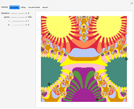
Snapshot 1: Exp-squared series, with  and
and  steps to show more detail. Changing the perturbation will vary the size, shape and position of the fractal-like patterns.
Snapshot 2: Sine-squared series, with  and
and  steps. Showing more steps will show more detail, and changing the perturbation will vary the size, shape and position of the fractal-like patterns.
Snapshot 3: Tangent series, with  and
and  steps. Changing the perturbation will vary the size of the fractal-like patterns, from points to circles that almost fill the entire shape.
References
[1] J. Bohman and C.-E. Föberg, "Heuristic Investigation of Chaotic Mapping Producing Fractal Objects," BIT Numerical Mathematics, 35, 1995 pp. 609–615. doi:10.1007/BF01739831.
[2] E. Kowalski and W. F. Sawin, "Kloosterman Paths and the Shape of Exponential Sums," Compositio Mathematica, 152(7), 2016 pp. 1489–1516. doi:10.1112/S0010437X16007351.
Permanent Citation
 Root-Finding Fractals
Enrique Zeleny Space-Filling Fractal Curves
Daniel de Souza Carvalho Fractal Popcorn
Enrique Zeleny Rauzy Fractals as Stepped Surfaces
Dieter Steemann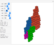 Rauzy Fractals of Order Four
Dieter Steemann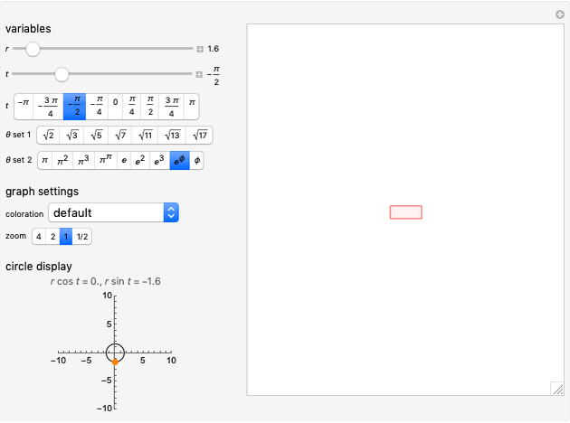 Julia Sets Produced by Cubic Polynomials
Xiaojun Jia, Troy Yang, Sarah Zimmerman and Efstathios Konstantinos Chrontsios Garitsis Generalized Cantor Sets and Their Hausdorff Dimensions
Erin K. Kline and Matthew A. Morena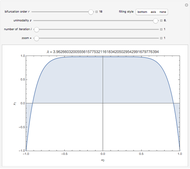 Iterates of Generalized Logistic Maps for Superstable Parameter Values
Ki-Jung Moon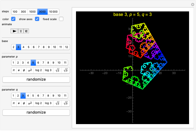 Fractal Curves Generated by the Sum-of-Digits Function
Adithya Swaminathan, Dimitrios Tambakos and A. J. Hildebrand Inflating a Dragon
Borut Levart
