Frequentist versus Bayesian PDF for Binary Decisions Like Coin Tossing, OSHA Compliance, and Jury Trials


Requires a Wolfram Notebook System
Interact on desktop, mobile and cloud with the free Wolfram Player or other Wolfram Language products.
The probability of success in a single trial  , the number of trials in an experiment
  , and the number of successful trials
  are the parameters used to illustrate both frequentist deductive reasoning and Bayesian inductive reasoning. The trials are independent and identically distributed (iid).


Contributed by: James C. Rock (July 2012)
Open content licensed under CC BY-NC-SA
Snapshots

Details
Discussion of Snapshots
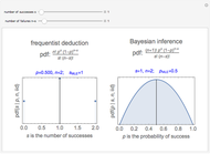
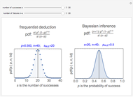
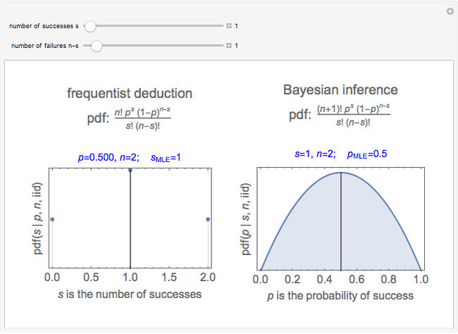
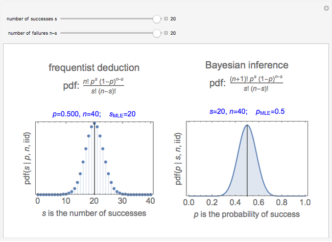
Snapshots 1 and 2 show the results from two experiments with  . The PDF is narrower for
  than it is for
  . Larger experiments lead to better precision.
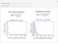
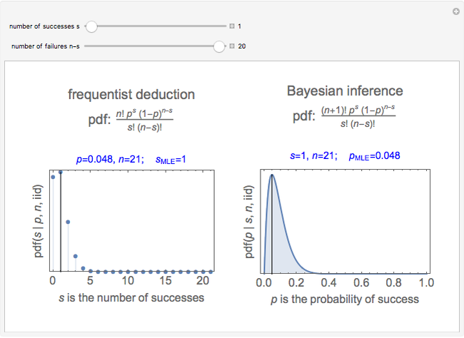
Snapshots 3 and 4 show the results from two extreme experiments, with 1 of 21 trials either failing or passing, resulting in  or
or  , respectively.
Snapshots 3 and 5 show results from two experiments with 1 failure in 21 or 6 trials, resulting in  or
or  , respectively.
Things to Try with This Demonstration
Examine the shape of  for
for  and for
  while takes values from 1 to 20. Note that the width of the PDF narrows as increases. This concept is useful for estimating the number of samples to plan for under anticipated experimental conditions.
Examine the shape of when for various between 1 and 20. Note again that the width narrows as increases.
You have now observed the reality of experimental design: to improve experimental precision one must dramatically increase the number of trials in an iid experiment.
Discussion
A binary trial, sometimes called a Bernoulli trial, is one that results in one of two outcomes, variously called success and failure, pass and fail, heads and tails, comply and non-comply, guilty and not guilty, 1 and 0, true and false. The terms success and fail or comply and non-comply are used in occupational and environmental compliance decisions.
An experiment consists of independent, identically distributed (iid) Bernoulli trials. The probability of success in each trial is , the probability of failure in the same trial is  , and is a real number in the closed interval
  .
.
Bayes's theorem is usefully expressed with likelihoods: posterior likelihood = prior likelihood × data likelihood. In this Demonstration, the prior likelihood function is the uninformative uniform distribution, so the posterior likelihood distribution = data likelihood distribution. The data likelihood for a binary experiment with iid trials is the product of the probabilities for each trial. In this Demonstration, the data likelihood is:
 .
.
This likelihood function (LHF) is the probability of any specific outcome from an experiment with trials yielding successes. It has three variables. Two of them ( and ) are known at the end of an experiment, while the third, , is not directly observed. The frequentist assumes a value for and deduces the discrete probability distribution for the number of successes in trials. The Bayesian, through Bayes's theorem, uses the data to infer the probability distribution for the parameter .
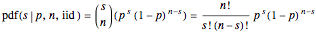
The frequentist uses the binomial coefficient to define the number of ways successes can be arranged among trials. Each of those arrangements has the same probability, which is denoted by  , ,
, ,  . The probability of is the product of the binomial coefficient and the probability of each individual arrangement of successes among sequential trials. In conditional probability notation (deprecated by some frequentist experts, but widely used by Bayesian experts), the resulting discrete binomial PDF is written:
 .
.
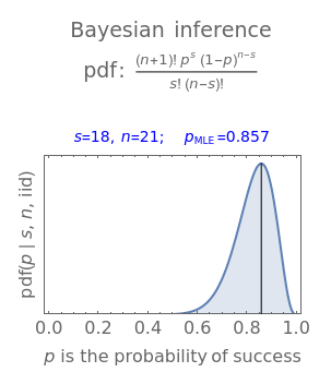
The Bayesian uses the data ( and ) to infer a conditional PDF for and to estimate its maximum likelihood value. The area under the likelihood function, here called the likelihood ( ), is calculated by integrating LHF with respect to over the range of 0 to 1. This is the Eulerian Integral, and it has a well-known solution:
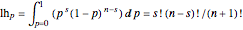 .
.
Divide the LHF by its area to find the functional form of the PDF with unit area:
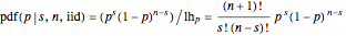 .
.
It turns out that both of these probability density functions can be expressed in terms of well-known parametric distributions. The first is the binomial distribution with independent variable , defined by parameters and . The second is the beta distribution with independent variable defined by shape parameters derived from and , so that  and
and . In Mathematica's notation these are expressed as:
 =PDF[BinomialDistribution[n, p], s] and
 =PDF[BetaDistribution[s+1, n-s+1], p]
To summarize, the likelihood function for a binomial experiment consisting of Bernoulli trials is central to both frequentist deduction and Bayesian inference. To the frequentist, LHF is the probability that an experiment ends with successes arranged in one of several sequences among trials. The probability of successes in trials, irrespective of the sequence, is expressed by counting the permutations of those trials. To the Bayesian, Bayes's theorem with the uniform distribution as the uninformative prior shows that LHF has the shape of the PDF of given and , and normalizing it to unit area produces the desired PDF.
This analysis produced two desired posterior distributions: the frequentist one for given and and the Bayesian one for given and . Suitable models for both of those distributions are found in the Mathematica collection of distributions. Using the binomial and beta distribution formalism opens the entire Mathematica spectrum of statistical analysis tools for further analysis of the compliance problem or any of its analogous binary decision problems.
References
[1] D. J. Blower, Information Processing: Boolean Algebra, Classical Logic, Cellular Automata, and Probability Manipulations, Pensacola, FL: David Blower, Third Millennium Inferencing, 2011.
[2] P. C. Gregory, Bayesian Logical Data Analysis for the Physical Sciences: A Comparative Approach with Mathematica® Support, New York: Cambridge University Press, 2010.
[3] D. Sivia and J. Skilling, Data Analysis: A Bayesian Tutorial, 2nd ed., New York: Oxford University Press, 2006.
[4] E. T. Jaynes, Probability Theory: The Logic of Science, New York: Cambridge University Press, 2003.
Permanent Citation
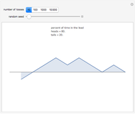 Leads in Coin Tossing
Fiona Maclachlan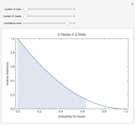 Maximum Likelihood Estimation for Coin Tosses
Tad Hogg Law of Large Numbers: Comparing Relative versus Absolute Frequency of Coin Flips
Paul Savory (University of Nebraska-Lincoln)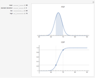 Connecting the CDF and the PDF
Roger J. Brown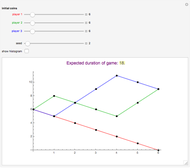 A Curious Coin-Flipping Game
Heikki Ruskeepää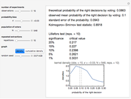 Kernel Density Estimations: Condorcet's Jury Theorem, Part 5
Tetsuya Saito Maximum Likelihood Estimators for Binary Outcomes
Seth J. Chandler Linear Dependence between Two Bernoulli Random Variables
Jeff Hamrick Comparing and Weighting Two Weibull Models
Frederick Wu Simulated Coin Tossing Experiments and the Law of Large Numbers
Ian McLeod