Numerical Example of One-Way ANOVA


Requires a Wolfram Notebook System
Interact on desktop, mobile and cloud with the free Wolfram Player or other Wolfram Language products.
This Demonstration illustrates some basic principles of one-way ANOVA (factor analysis of variance) and shows how it works so you can analyze the statistical variability of a statistical complex.
[more]
Contributed by: Olexandr Eugene Prokopchenko and Pylyp Prokopchenko (September 2012)
Open content licensed under CC BY-NC-SA
Snapshots


Details
In ANOVA logic, partitioning the sources of variance and hypothesis testing can be done individually. According to the ANOVA method, the total variation is decomposed into two parts: a source of variation due to the group or factor effect (expressed with  ) and a source of variation due to the measurement error (expressed with
  ).
).
This Demonstration uses the ANOVA table algorithm based on deviations.
By definition, the variance  , where
  is the sum of squared deviations;
  is the total deviation, based on the differences between variants
  and the mean of statistical complex; is the intergroup or between-group deviation, based on differences between each group (or sample) and the complex means; and is the intragroup or within-group deviation, based on differences between the variants and the sample (group) mean.
This Demonstration illustrates some basic principles of one-way ANOVA only. We know that the Fisher  -test is used for comparisons of the components of the total deviation. The -value is the ratio of variance between and variance within samples (groups).
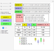
Consider an experiment to study the effect of three different levels of a factor on a response  ,
,  ,
,  . With
  (here we use
  but say there are
  groups) observations for each level, we write the outcome of the experiment in a work table.
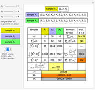
To calculate the -ratio:
Calculate the size of the statistical complex (first row in the work table)  .
.
Calculate the sum  within each sample (group), and the complex total sum
 , adding values in the row.
Calculate  , the square of the sum.
Find the value  and the total sum in the row:
 .
.
Calculate the  (sum of square).
Find the total sum in the row  .
.
Find the value  :
:

and the deviations:
 ,
,
 ,
,
 .
.
Calculate total variance  , between-group variance
  , and within-group variance
  .
.
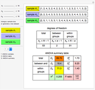
The statistical ANOVA complex degrees of freedom is  .
.
The between-group degrees of freedom is one less than the number of groups (samples):  .
.
The within-group degrees of freedom is  .
.
And finally we find the -ratio:

and the relative factor effect:
 .
.
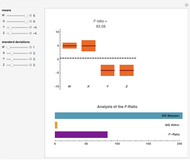
It is well known that the -test is used to compare the components of the total deviation. In this Demonstration, we are using the textbook method of concluding the hypothesis test: compare the observed -value with the critical value of determined from tables. The critical value of is a function of the numerator degrees of freedom, the denominator degrees of freedom, and the significance level alpha. If the experimental -value is more than critical -value, then reject the null hypothesis.
The Demonstration has thus illustrated how we can get and apply the experimental -value.
References
[1] A. Gelman, "Analysis of Variance—Why It Is More Important Than Ever," Annals of Statistics, 33(1), 2005. pp. 1–53. doi:10.1214/009053604000001048.
[2] D. C. Montgomery, Design and Analysis of Experiments, 5th ed., New York: Wiley, 2001.
Permanent Citation
 Visual ANOVA
Francois Giraud-Carrier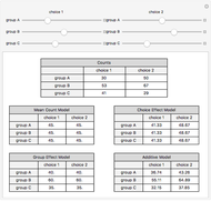 Comparing Models for Two-Way Contingency Tables
Darren Glosemeyer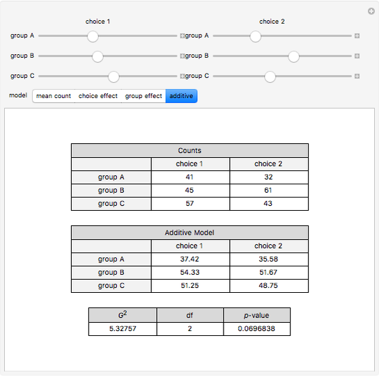 Likelihood-Based Goodness of Fit in Two-Way Contingency Tables
Darren Glosemeyer The Method of Common Random Numbers: An Example
Jeff Hamrick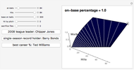 Baseball: Graph of On-Base Percentage
Danny Strockis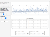 Cumulative Sums and Visual Change Detection between Two Random Processes
Olexandr Eugene Prokopchenko and Pylyp Prokopchenko 1, 2, 3-Parameter Logistic Rasch and Birnbaum Models and Item Analysis
Olexandr Eugene Prokopchenko The Envelope Theorem: Numerical Examples
Jeff Hamrick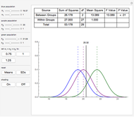 Single Factor Analysis of Variance
Scott R. Colwell Law of Large Numbers: Dice Rolling Example
Paul Savory (University of Nebraska-Lincoln)
