Three Alternatives to the Likelihood Maximization for Estimating a Centered Matérn (3/2) Process


Requires a Wolfram Notebook System
Interact on desktop, mobile and cloud with the free Wolfram Player or other Wolfram Language products.
This Demonstration is restricted to the case of no measurement error. In the Demonstration mentioned in the last paragraph, the exact maximum-likelihood (ML) method is implemented for this case (indeed the exact minimizer is then explicit for the Ornstein–Uhlenbeck case). In this Demonstration, an exact ML method is not implemented because, in spite of the existence of a fast order- algorithm to compute the likelihood criterion, its global maximization (even for its "profile" version) is not an easy task, unless one is content to find an approximate solution by a rough grid search.


Contributed by: Didier A. Girard (January 2015)
(CNRS-LJK and Université Grenoble Alpes)
Open content licensed under CC BY-NC-SA
Snapshots

Details
It can be shown (e.g. in the Papoulis book cited in [1]) that the stationary solution of the above second-order SDE is a centered Gaussian process whose autocorrelation function has the simple expression 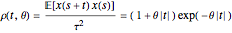 , which is the more classical definition of a Matérn (3/2) process (here
  denotes the ensemble averaging, i.e. from infinitely repeated simulations of the process under the true model).
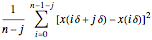
By choosing equispaced abscissae, the simulations are greatly facilitated, since the observations then coincide to a particular ARMA(2,1) time series, the transformation giving the ARMA parameters from  and
and  requiring only simple and well-known computations [7].
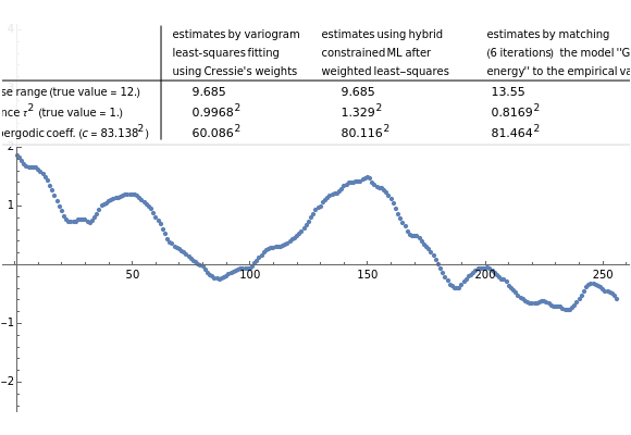
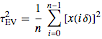
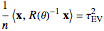
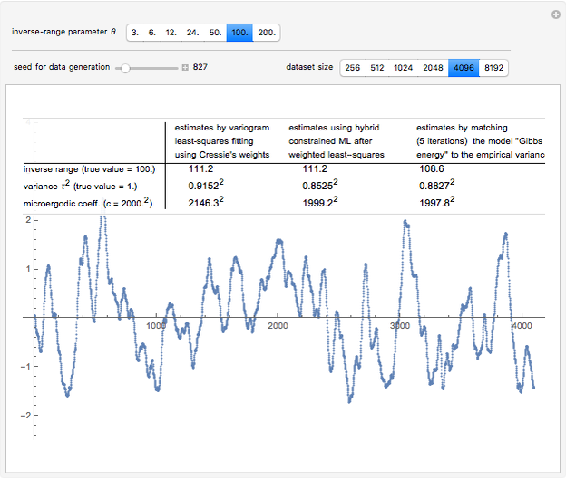
For all the simulated time series, the variance  is fixed to 1, called "true (unknown) value of variance" (this choice is without loss of generality), and various can be tried for the true value of the inverse-range parameter. The resulting true value for the microergodic parameter
  is displayed at the bottom-left (third line) of the table of the numerical results.
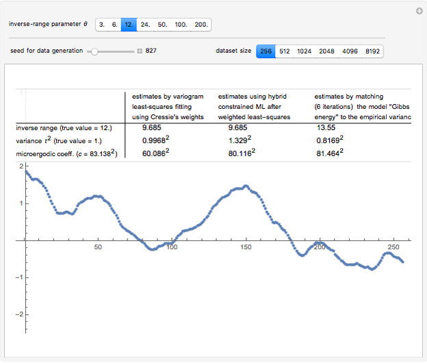
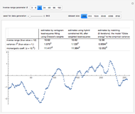
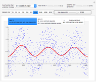
Snapshot 1: Selecting 12 as the true inverse-range parameter and  , you can first compare the estimates produced by the classical variogram least-squares fitting (first column) versus Zhang and Zimmerman hybrid estimates (second column; note that the estimate of is also displayed in this second column, even though it is unchanged from the first column): for this seed (827), the variance estimate (second line) is observed to be degraded by the hybrid method, but the estimate of is much improved. Looking now at the third column, which displays the results produced by the third estimation method, CGEM-EV, you observe an improvement for the estimate of and a little change for the estimate of , as compared to the hybrid method.
By changing the seed (and thus a new  is used to generate the data), you can be convinced that these remarks about the three estimates of are not an accident. But you can also observe a rather large variability (i.e. from seed to seed) for each of the three estimates of the variance (or of ); this is much larger than the variability of the estimates of the microergodic coefficient , which can be observed for the hybrid or CGEM-EV methods. Notice that this observation is in very good agreement with the known theory about the estimation of the variance, the inverse-range parameter, and their product (see [6], [3], [2] and the references therein).
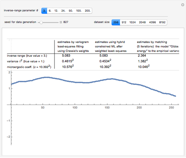
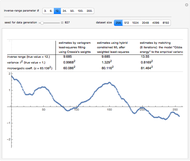
Snapshot 2: Now selecting 3 as true , a clear improvement (in the estimation of or of ) by using CGEM-EV in place of the hybrid method can be observed: indeed, for such "large range" settings, the least-squares fitting method produces even more variable estimates (and it often produces estimates at the boundary of the grid search, here 1.5). Increasing (for example, setting  ), you can observe that the estimate of is also improved, although to a lesser extent.
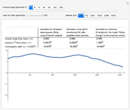
Snapshot 3: Staying at and now selecting 100 as true (this is a "rather small range" setting), a ranking of CGEM-EV and the hybrid method based on their statistical performances becomes much more difficult. One also observes that the relative accuracy of both these estimates of or of is clearly increased as compared to the above "large range" settings.
References
[1] C. E. Rasmussen and C. K. I. Williams, Gaussian Processes for Machine Learning, Cambridge, MA: MIT Press, 2006. www.gaussianprocess.org/gpml/chapters.
[2] H. Zhang, "Asymptotics and Computation for Spatial Statistics," in Advances and Challenges in Space-time Modelling of Natural Events (Lecture Notes in Statistics, Vol. 207) (E. Porcu, J. M. Montero, and M. Schlather, eds.), New York: Springer, 2012 pp. 239–252. doi:10.1007/978-3-642-17086-7_10.
[3] C. G. Kaufman and B. A. Shaby, "The Role of the Range Parameter for Estimation and Prediction in Geostatistics," Biometrika, 100(2), 2013 pp. 473–484. doi:10.1093/biomet/ass079.
[4] N. Cressie, "Fitting Variogram Models by Weighted Least Squares," Journal of the International Association for Mathematical Geology, 17(5), 1985 pp. 563–586. doi:10.1007/BF01032109.
[5] H. Zhang and D. L. Zimmerman, "Hybrid Estimation of Semivariogram Parameters," Mathematical Geology, 39(2), 2007 pp. 247–260. doi:10.1007/s11004-006-9070-8.
[6] D. A. Girard, "Asymptotic Near-Efficiency of the 'Gibbs-Energy and Empirical-Variance' Estimating Functions for Fitting Matérn Models to a Dense (Noisy) Series." arxiv.org/abs/0909.1046v2.
[7] M. S. Phadke and S. M. Wu, "Modeling of Continuous Stochastic Processes from Discrete Observations with Application to Sunspots Data," Journal of the American Statistical Association, 69(346), 1974 pp. 325–329. www.jstor.org/stable/2285651.
Permanent Citation
 Estimating a Centered Ornstein-Uhlenbeck Process under Measurement Errors
Didier A. Girard Nonparametric Additive Modeling by Smoothing Splines: Robust Unbiased-Risk-Estimate Selector and a Nonisotropic-Smoothing Improvement
Didier A. Girard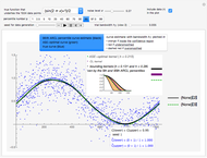 Nonparametric Regression and Kernel Smoothing: Confidence Regions for the L2-Optimal Curve Estimate
Didier A. Girard Hypothesis Tests about a Population Mean
Chris Boucher Distribution of Discrete Records
Heikki Ruskeepää Records in Sequences of Random Variables
Heikki Ruskeepää Edgeworth Expansion for Near-Normal Data
Housam Binous, Mamdouh Al-Harthi, and Brian G. Higgins The Power of a Test Concerning the Mean of a Normal Population
Chris Boucher Distributions of Order Statistics
Chris Boucher Polynomial Fits of Random Walks
Michael Schreiber
-
 Nonparametric Density Estimation: Robust Cross-Validation Bandwidth Selection via Randomized Choices
Didier A. Girard -
Nonparametric Additive Modeling by Smoothing Splines: Robust Unbiased-Risk-Estimate Selector and a Nonisotropic-Smoothing Improvement
Didier A. Girard -
 Nonparametric Curve Estimation by Smoothing Splines: Unbiased-Risk-Estimate Selector and its Robust Version via Randomized Choices
Didier A. Girard -
Estimating a Centered Ornstein-Uhlenbeck Process under Measurement Errors
Didier A. Girard -
 Estimating a Centered Matérn (1) Process: Three Alternatives to Maximum Likelihood via Conjugate Gradient Linear Solvers
Didier A. Girard -
 Three Alternatives to the Likelihood Maximization for Estimating a Centered Matérn (3/2) Process
Didier A. Girard -
Nonparametric Regression and Kernel Smoothing: Confidence Regions for the L2-Optimal Curve Estimate
Didier A. Girard -
 Nonparametric Curve Estimation by Kernel Smoothers: Efficiency of Unbiased Risk Estimate and GCV Selectors
Didier A. Girard