Restricted Three-Body Problem

Requires a Wolfram Notebook System
Interact on desktop, mobile and cloud with the free Wolfram Player or other Wolfram Language products.
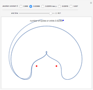
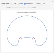
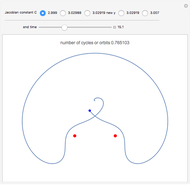
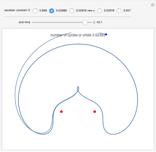
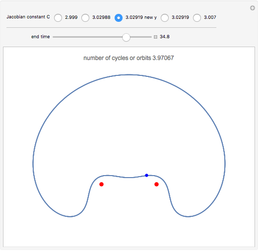
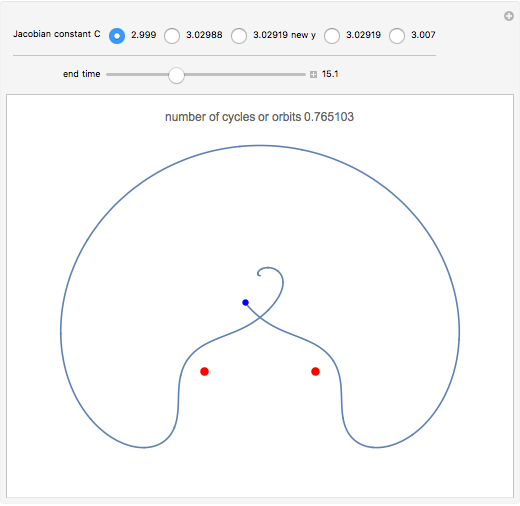
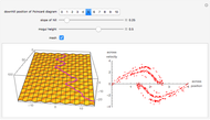
The red dots represent two equal masses that rotate around each other to maintain their spacing. The axes rotate so that these masses appear to be stationary. The blue dot represents the third body, which has negligible (zero) mass. This third body is initially on the  axis and has an initial velocity in the
  direction. The number of orbits is shown in the window.
Contributed by: Robert M Lurie (March 2011)
Additional contributions by: Szabolcs Horvát
Open content licensed under CC BY-NC-SA
Snapshots
Details
This is a modification of the Demonstration Restricted Three-Body Problem in 3D (see Related Links) that shows several 2D classical orbits based on those in F. R. Moulton, Periodic Orbits, Washington, D.C.: Carnegie Institution of Washington, 1920.
Moulton characterized the orbits of this system by their Jacobian constant  . The starting values given here are from V. Szebehely and T. van Flandern, "A Family of Retrograde Orbits around the Triangular Equilibrium Points," Astronomical Journal, 72, 1967 p. 373.
The restricted three-body problem is clearly discussed in section 2.9 of the wonderful book by R. Gass, Mathematica for Scientists and Engineers, Upper Saddle River, NJ: Prentice-Hall, 1998. This should be read by anyone interested in the details of this problem.
The starting values were extended by running the program for longer orbit times and modifying the values to keep the orbits stable. Moulton starts with values for the initial velocity in the direction and the value at zero for each; he then assigns initial values for the velocity in the direction and the location. The values in Moulton or in Szebehely and van Flandern will give a partial or only a slight reproduction in the orbits. By using the high-precision capabilities of Mathematica one may extend the initial values of either the velocity in the direction or the location and find that one may obtain three or more "stable" cycles. This is analogous to balancing a pencil on its tip. In the examples given here, the initial direction velocity is extended by trial and error except for one  where the initial value is extended.
Permanent Citation
 Restricted Three-Body Problem in 3D
Enrique Zeleny The Celestial Two-Body Problem
S. M. Blinder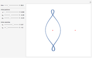 Restricted Three-Body Problem in a Plane
Enrique Zeleny Mass Transfer in Binary Star Systems
Jeff Bryant Three-Body Problem in 3D
Jeff Bryant and José Martin?Garcia Planar Three-Body Problem
Michael Trott Planar Three-Body Problem in Phase Space
Michael Trott Choreographic Motions of N Bodies
Robert M Lurie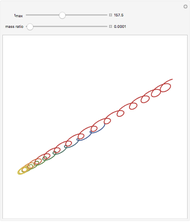 Orbits around the Lagrange Point L4
Enrique Zeleny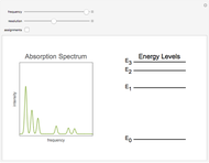 Absorption Spectroscopy
S. M. Blinder
-
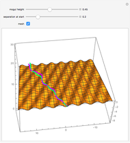 Chaos While Sledding on a Bumpy Slope
Robert M Lurie -
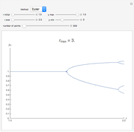 Numerical Integration of the Logistic Equation Using Runge-Kutta Methods
Robert M Lurie -
 Sledding on a Bumpy Slope: Chaos and Strange Attractor
Robert M Lurie -
 Classic Logistic Map
Robert M Lurie -
 Restricted Three-Body Problem
Robert M Lurie -
Choreographic Motions of N Bodies
Robert M Lurie