Stock Price Probability with Stable Distributions


Requires a Wolfram Notebook System
Interact on desktop, mobile and cloud with the free Wolfram Player or other Wolfram Language products.
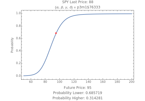
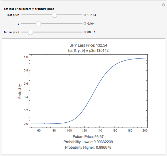
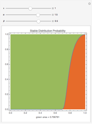
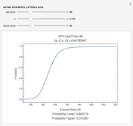
This Demonstration calculates the probability that the random price of the exchange-traded fund, SPY, will be higher or lower after one month than a particular future possibility.
[more]


Contributed by: Bob Rimmer (March 2011)
Open content licensed under CC BY-NC-SA
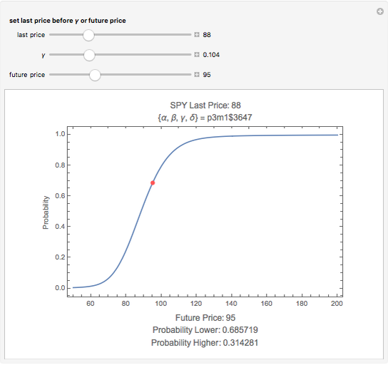
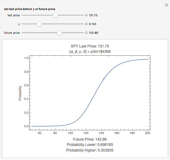
Snapshots


Details
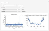
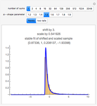
Levy-stable distributions were introduced for financial returns by Mandelbrot in 1963. They offer an advantage over the log normal assumption in that extreme events can exist in the model. They have not been in much use because of the difficulty in performing the calculations. Most models using stable distributions have also assumed that they are stationary; when parameters are fitted to a stationary stable model, the tails are consistently found to be too heavy. The parameters for the particular example were scaled from intraday observations at one-minute intervals. The parameters chosen for the example were obtained by maximum-likelihood fitting (using an FFT approximation of the stable density from the sampled stable characteristic function) over six months of data, after rescaling each day's data by a value of  derived from an empirical characteristic fit. This method removes most of the serial dependence seen in the data and gives a value of
  that is significantly higher than would be found by fitting the raw data, assuming the distribution is stationary. The parameters and
  are selected from average days, but the user needs to be aware that may vary by a factor of 2 or 3 during volatile periods in the market. The user who downloads the source may experiment with his own parameters.
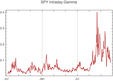
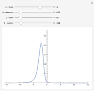
Since this graphic was first put up the stock market has demonstrated some remarkable behavior. Below is a plot of intra-day gamma calculations from July 2007 to mid December 2008, rescaled to one month to help in guessing the gamma parameter for the future. This new version of this Demonstration allows the user to adjust the gamma parameter as a measure of volatility in the market.
Software is now available for Mathematica that can do the parameter fitting and other calculations. This Demonstration uses only a fragment of the free software available at mathestate, where there is a growing series of web pages devoted to the financial applications of stable distributions, including a nonstationary stable model.
Permanent Citation
 Stock Price Simulation Using Stable Random Variables
Bob Rimmer Stable Distribution Function
Bob Rimmer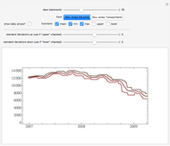 Stock Price Envelopes
Seth J. Chandler Logistic Sigmoid Market Model
Michael Schreiber Tail Conditional Expectations
Seth J. Chandler Power Law Tails in Log Normal Data
Fiona Maclachlan The Return Distribution of the Variance Gamma Process
Andrzej Kozlowski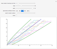 Simulating the Poisson Process
Heikki Ruskeepää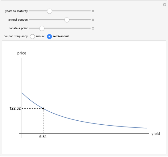 Price-Yield Curve
Fiona Maclachlan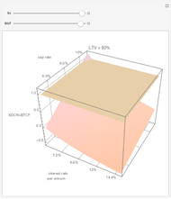 Explaining Real Estate Price Bubbles
Roger J. Brown
-
Stock Price Simulation Using Stable Random Variables
Bob Rimmer -
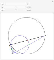 Nine-Point Circle in the Complex Plane
Bob Rimmer -
 Generalized Central Limit Theorem
Bob Rimmer -
Stable Distribution Function
Bob Rimmer -
 Stable Distribution Computed with the Zolotarev Integral
Bob Rimmer -
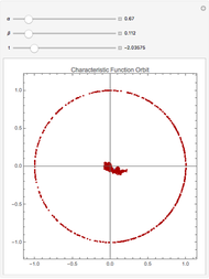 Empirical Characteristic Function
Bob Rimmer -
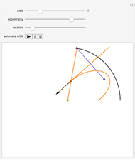 Newton's Ellipse
Bob Rimmer -
 Stock Price Probability with Stable Distributions
Bob Rimmer -
 Stable Density Function
Bob Rimmer