Tracking an Object in Space Using the Kalman Filter


Requires a Wolfram Notebook System
Interact on desktop, mobile and cloud with the free Wolfram Player or other Wolfram Language products.
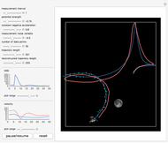
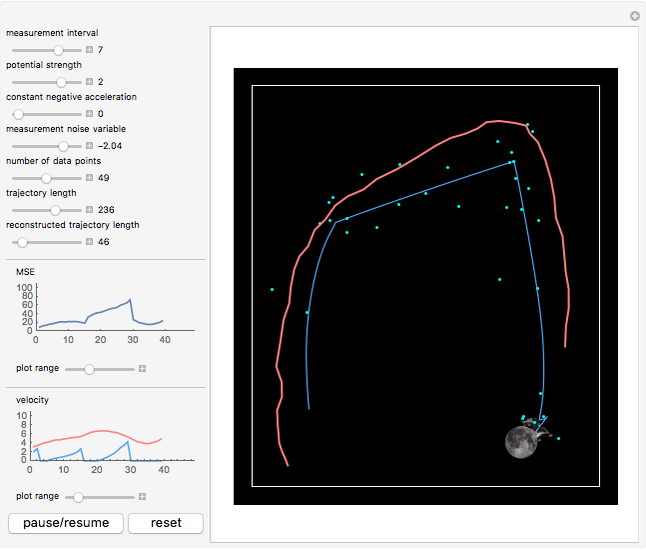
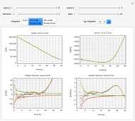
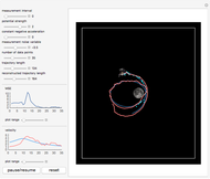
Tracking an object in space using the Kalman filter can reconstruct its trajectory and velocity from noisy measurements in real time. The object, indicated by a blue pentagon, undergoes motion in a gravitational  potential of adjustable magnitude created by an external mass, chosen as the Moon, whose position you can control by dragging. The boundary conditions at the box edge are reflective.
Contributed by: Oliver K. Ernst (July 2015)
Open content licensed under CC BY-NC-SA
Snapshots

Details
Snapshot 1: the filtered trajectory and velocity are reconstructed in real time
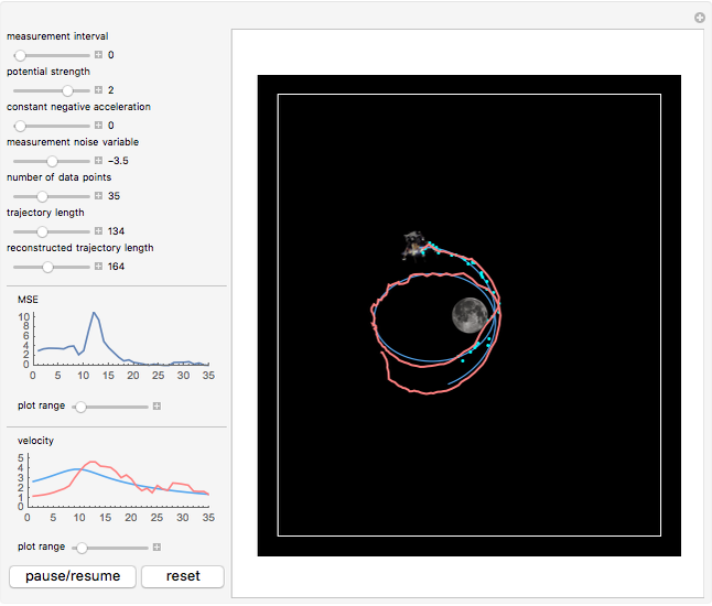
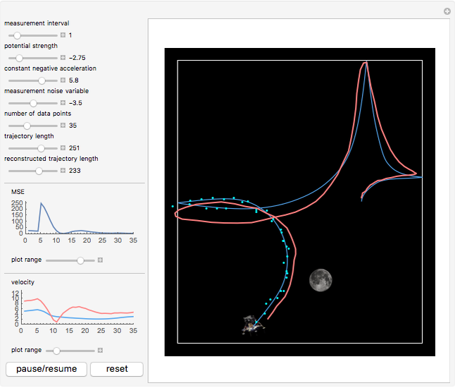
Snapshot 2: at high measurement noise and long measurement interval, the accuracy of the filter deteriorates
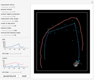
Snapshot 3: it is possible to adjust the magnitude of the gravitational potential to be repulsive (negative), as well as to include an optional constant deceleration
The object (lunar module [1]) undergoes motion in a gravitational field, experiencing an acceleration
 .
.
Here,  is the vector from the Moon [2] to the object,
  is the strength of the potential, which you can vary to be either positive (attractive) or negative (repulsive), and
  is a constant acceleration in the direction opposite the velocity of the object, which you can also vary. In the case of a collision between the object and the Moon, the object is stopped on the lunar surface; the walls of the box are reflective.
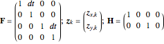
The Kalman filter is used to reconstruct the position and velocity of the object from noisy position measurements. For a detailed description of the Kalman filter, see e.g. [3, 4, 5]. Following the notation in [3], the model for the object's discrete time evolution can be expressed as
 ,
,
 ,
,
where  denotes the state vector,
  denotes the noisy position measurements made,
  is the process noise,
  is the measurement noise, and
 ;
;  .
.
The measurement noise covariance matrix is assumed to be known:
 ,
,
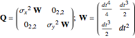 ,
,
where  is the variance of the
  component of the acceleration, and similarly for
  . The variances are determined from a sample of the true accelerations experienced by the object (with sample size equal to the variable number of data points), although in practice this information is not available and other methods must be employed (see e.g. [6]).
To determine the performance of the filter, the MSE  , where
  is the true state vector of the object, is updated at each time step, whose expectation value is minimized by the filter.
References
[1] NASA. "Apollo 11 Lunar Module Eagle in Landing Configuration in Lunar Orbit from the Command and Service Module Columbia." (Jun 30, 2015) commons.wikimedia.org/wiki/File:Apollo_ 11_Lunar _Module _Eagle _in _landing _configuration _in _lunar _orbit _from _the _Command _and _Service _Module _Columbia.jpg.
[2] G. H. Revera. "High Resolution Photo of Completely Full Moon." (Jun 30, 2015) commons.wikimedia.org/wiki/Moon#/media/File:FullMoon2010.jpg.
[3] Wikipedia. "Kalman Filter." (Jun 30, 2015) en.wikipedia.org/wiki/Kalman_filter.
[4] E. Cuevas, D. Zaldivar, and R. Rojas, Kalman Filter for Vision Tracking, Technical Report B 05-122005, Freie Universität Berlin and Institut für Informatik and Universidad de Guadalajara, 2005. www.diss.fu-berlin.de/docs/servlets/MCRFileNodeServlet/FUDOCS_derivate_ 000000000473/2005_ 12.pdf.
[5] R. E. Kalman, "A New Approach to Linear Filtering and Prediction Problems," Transactions of the ASME Journal of Basic Engineering, 82(1, Series D), 1960 pp. 35-45. doi:10.1115/1.3662552.
[6] F. V. Lima. "Autocovariance Least-Squares (ALS) Package." (Jun 30, 2015) jbrwww.che.wisc.edu/software/als/index.html.
Permanent Citation
 Tuning an Extended Kalman Filter
Brian C. Beckman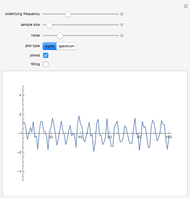 Frequency Spectrum of a Noisy Signal
Jon McLoone Analog-to-Discrete System Conversion Using Impulse Invariance
Nasser M. Abbasi Sine Wave Generation Using an Unstable IIR Filter
Charles Masenas Pi Filter
Selwyn Hollis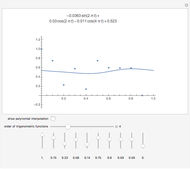 Trigonometric Fitting and Interpolation
Bruce Atwood and Rikley Buckingham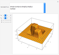 XFT2D: A 2D Fast Fourier Transform
Rafael G. Campos, J. Jesus Rico Melgoza, and Edgar Chavez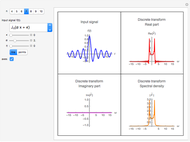 XFT: An Improved Fast Fourier Transform
Rafael G. Campos, J. Jesus Rico Melgoza, and Edgar Chavez Lowpass Filter Design by Pole Placement
Aaron T. Becker Response of Low-Pass RC Filter to Periodic Waveforms
Mariusz Jankowski
-
 Pattern Formation in the Kuramoto Model
Oliver K. Ernst -
 Gillespie's Stochastic Simulation Algorithm for Chemical Reactions
Oliver K. Ernst -
 Electrodiffusion of Ions across a Neural Cell Membrane
Oliver K. Ernst -
 Action Potential Propagation along Myelinated Axons
Oliver K. Ernst -
 Picard's Method for Ordinary Differential Equations
Oliver K. Ernst -
 Distributions Using Slice Sampling
Oliver K. Ernst -
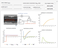 The Hodgkin-Huxley Experiment on Neuron Conductance
Oliver K. Ernst -
 Tracking an Object in Space Using the Kalman Filter
Oliver K. Ernst -
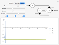 Feedforward and Feedback Control in Neural Networks
Oliver K. Ernst