Two-Dimensional Cellular Automata from One-Dimensional Rules


Requires a Wolfram Notebook System
Interact on desktop, mobile and cloud with the free Wolfram Player or other Wolfram Language products.
Some nontrivial two-dimensional (2D) cellular automata (CA) are reproduced with one-dimensional (1D) CA rules. Thus a large subclass of 2D CA can be conveniently labeled through the standard Wolfram indexing of 1D CA. One step of time evolution of a 2D CA is obtained in two stages. First, apply a 1D rule to all the ROWS of a 2D initial condition. Then to the result apply another 1D rule, but now to all the COLUMNS. Here this procedure is repeated 500 times, generating the evolution of a random 2D initial condition for 500 steps. This can be mapped onto the subclass of  two-color 2D CA with a nine cell square neighborhood. It is useful to devise smaller subclasses of the general case to manage classification of such a large number of CA. Examples of such subclasses are totalistic CA, outer-totalistic CA, and the new subclass demonstrated here. Browse and animate bookmarks for interesting patterns. See the Details section for more a extensive explanation of the controls and images.
Contributed by: Vitaliy Kaurov (March 2011)
Open content licensed under CC BY-NC-SA
Snapshots

Details
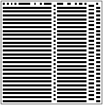
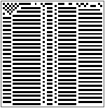
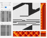
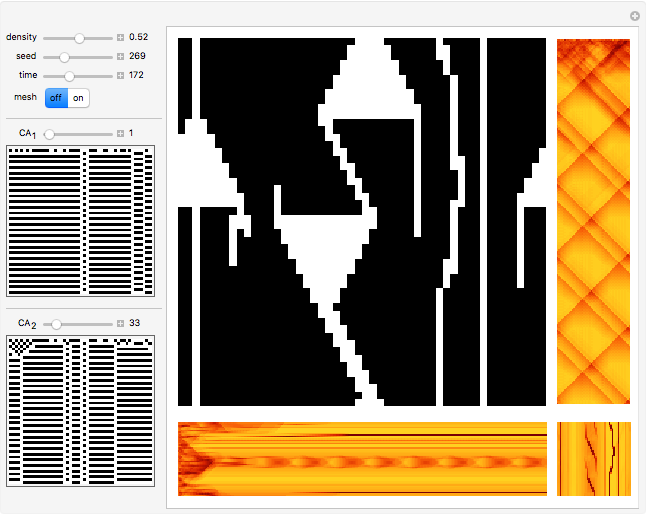
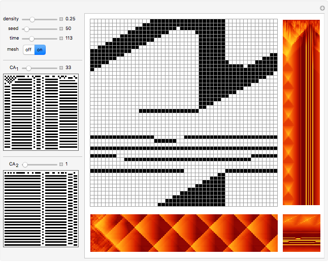
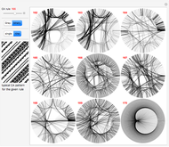
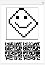
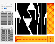
The two black-and-white (B&W) images in the control area on the left are random samples of 1D CA rules applied during two stages described in the caption. Their patterns do not directly participate in the creation of images on the right and are given for general reference and comparison only. Evolution time runs from top to bottom. Rules and their patterns are set by the controls  and
and  .
.
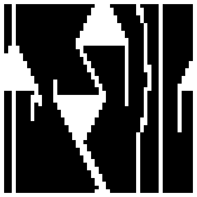
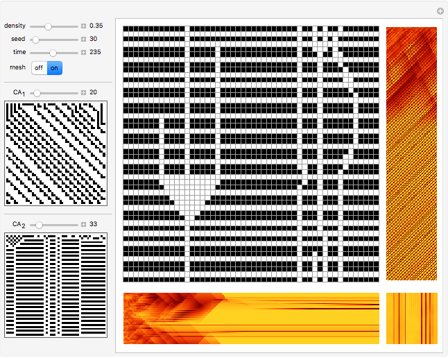
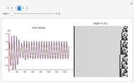
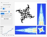
The large B&W square image on the right represents a particular step in the time evolution of a random 2D initial condition (50 by 50 cells). Choose these time steps with the time control. Randomize the initial condition with the seed control. Choose the density of black cells in the initial condition with the density control.
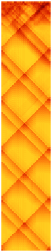
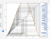
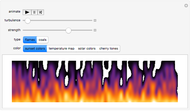
Solar-colored vertical rectangle:
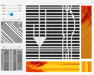
The values of the cells in the large B&W square are averaged in every row, thus producing a 50-element vector of averages for every time step. The first 250 such vectors are plotted with time running from top to bottom. If there are robust structures moving vertically in a 2D CA (hence vertical orientation of image), they will show as inclined lines on such a plot, as can be seen in snapshot 1.
Solar-colored horizontal rectangle:
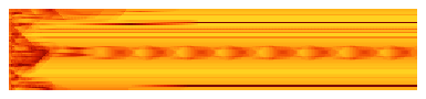
The values of cells in the large B&W square are averaged in every column, thus producing a 50-element vector of averages for every time step. The first 250 such vectors are plotted with time running from left to right. If there are robust structures moving horizontally in a 2D CA (hence horizontal orientation of image), they will show as inclined lines on such a plot, as can be seen in snapshot 2.
The small solar-colored square at the bottom-right corner is the time average of all 500 evolution steps.
Snapshot 1: triangular structures in the large B&W square are moving vertically in opposite directions (vary the time control to see the motion); this shows up as crossing slanted lines in the vertical solar-colored rectangle
Snapshot 2: counter-horizontally moving structures in the large B&W square show up as crossing slanted lines on the horizontal solar-colored rectangle; vary the time control to see the motion
Snapshot 4: different structures move horizontally with different speeds (vary the time control to see the motion); hence slanted lines have different slopes in the horizontal solar-colored rectangle
Snapshot 5: motion in perpendicular directions can be noticed; change the time control to see the motion
Permanent Citation
 Cellular Automata Coupled by Overlap or Common Boundary
Vitaliy Kaurov Cobweb Diagrams of Elementary Cellular Automata
Vitaliy Kaurov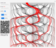 Order, Chaos, and the Formation of a Cantor Set Attractor in Elementary Cellular Automata
Vitaliy Kaurov One-Dimensional Cellular Automata on the Regular Tessellations
Machi Zawidzki Two-Dimensional Recursive Subdivision of the Evolution of a Cellular Automaton
Abigail Nussey Patterns from the Mean of Two-Color Totalistic 2D Cellular Automata
Daniel de Souza Carvalho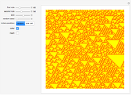 Flipping between Two Elementary Cellular Automaton Rules
Daniel de Souza Carvalho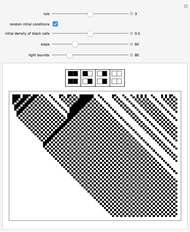 Two-Color Block Cellular Automata
Abigail Nussey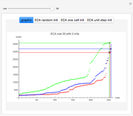 Elementary Cellular Automata Rules with Different Initial Conditions
Daniel de Souza Carvalho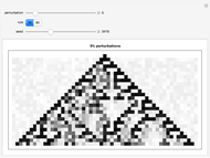 Randomized Evolutions of Continuous Cellular Automata Generalizing Rules 30 and 90
Abigail Nussey
-
 Constrained Optimal Routes in 3D Space
Vitaliy Kaurov -
 Iconography for Elementary Cellular Automata Based on Radial Convergence Diagrams
Vitaliy Kaurov -
Order, Chaos, and the Formation of a Cantor Set Attractor in Elementary Cellular Automata
Vitaliy Kaurov -
Cobweb Diagrams of Elementary Cellular Automata
Vitaliy Kaurov -
 Time Series and Cobwebs for Arbitrary Recursive Maps on the Unit Interval
Vitaliy Kaurov -
 Peter de Jong Attractors
Vitaliy Kaurov -
 Horizontal Visibility Graphs for Elementary Cellular Automata
Vitaliy Kaurov -
 Digital Representation of a Nonlinear ODE with Small Differences in Initial Conditions
Vitaliy Kaurov -
 Two-Dimensional Block Cellular Automata with a 2×2 Neighborhood
Vitaliy Kaurov -
 Single-Share Password-Protected Visual Cryptography via Cellular Automata
Vitaliy Kaurov -
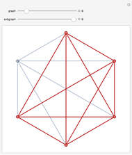 Random Subgraph of a Complete Graph
Vitaliy Kaurov -
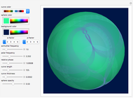 Lissajous Patterns on a Sphere Surface
Vitaliy Kaurov -
Cellular Automata Coupled by Overlap or Common Boundary
Vitaliy Kaurov -
 Two-Dimensional Cellular Automata from One-Dimensional Rules
Vitaliy Kaurov -
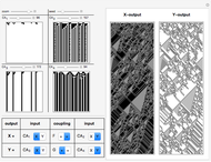 Coupled Cellular Automata: Symbiotic Patterns and Synchronization
Vitaliy Kaurov -
 Simulating Flickering Fire with Noisy Cellular Automaton
Vitaliy Kaurov