Estimating a Centered AR1 x AR1 Gaussian Field by Likelihood Maximization or GE-EV Matching

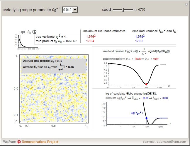
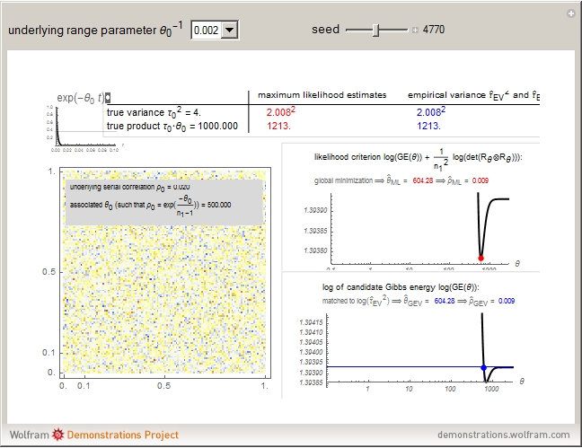
Every stationary Gaussian random field , where , is determined by its constant mean ( when the field is assumed centered), its variance and its autocorrelation function , which satisfies:

, where and .

This Demonstration considers a well-studied example of such a field, defined by:

,

which might be considered a simple extension of the well-known Ornstein–Uhlenbeck (OU) process to two dimensions. This random field is also called the OU sheet. As in one dimension, is often called the range parameter. See [1, 2] and [3, Chap. 12] for plots of the Brownian sheet, which is a limit version (as ) of the OU sheet. Note that horizontal and vertical features are well present in an OU sheet, especially for small .

To simplify, let us assume that one realization of such a field is observed on the regular grid with and .

If the observed image (whose entry is ) is rearranged in a vector of size by stacking its columns, it can be checked that is a Gaussian vector whose covariance matrix coincides with the Kronecker product

,

where denotes the correlation matrix of an AR(1) time series of parameter (precisely, its serial correlation being ). Such an image is also said to be an process.

Simulating such a is quite fast (see Details). Here this can be done once a value for the underlying range parameter is chosen in a list of values similar to the one in Table 3 of [4], except that some smaller values are added.

It is well known that the classic maximum likelihood (ML) principle can be easily implemented, even for large , by using the known expression of (a tridiagonal matrix) and its determinant and by exploiting the properties of the Kronecker product. It can be verified here that the calculation of the profile log-likelihood is very fast even when computed over a fine grid of -values: this criterion (up to a constant term) multiplied by is displayed in the top-right panel for each simulated .

This Demonstration also studies the "energy variance matching" alternative to ML (GE-EV method, which is the "no-noise" version of CGEM-EV), which was already implemented in a series of Demonstrations for different contexts in the one-dimensional case (Matérn autocorrelations and the powered-exponential autocorrelation). Recall that it consists of first taking the naive empirical variance as an estimate of , next defining by matching the quadratic form

, where ,

here (the so-called "candidate Gibbs energy of " denoted ) to . Of course (since GE-EV requires even fewer computations than ML) the implementation of GE-EV is also very fast (bottom-right panel).

As observed in [4] for isotropic random fields, ML and GE-EV methods give quite close results except for settings with a large range. For these extreme settings, the proximity of the two methods is restored provided we only focus on the estimation of the product , which plays here the role of a micro-ergodic coefficient (see [5]), as was the case for the diffusion coefficient specific to each of the above-mentioned one-dimensional cases.