Sensitivity to Initial Conditions for the Logistic Map


Requires a Wolfram Notebook System
Interact on desktop, mobile and cloud with the free Wolfram Player or other Wolfram Language products.
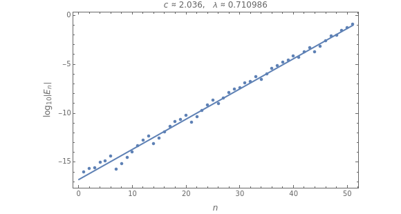
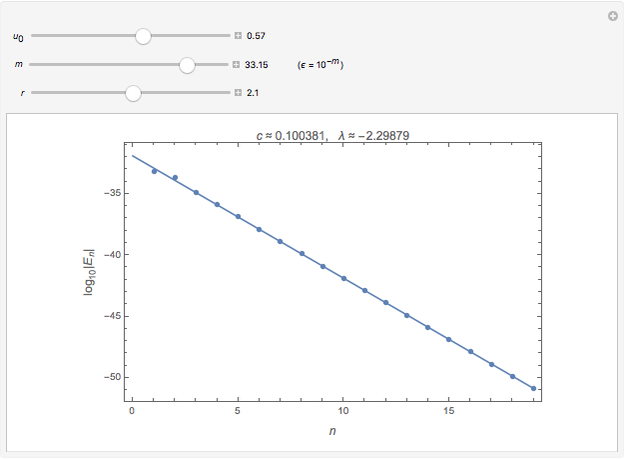
This Demonstration shows the evolution of the distance  between two orbits of the logistic map
  , where
  or
or  . The two orbits are initially separated by a perturbation of size
  . The plot is of
  versus
  for an orbit starting at
  , perturbation
  and parameter
  . An estimate of the error amplification factor
  and the Lyapunov exponent
  are shown at the top of the graphic.
Contributed by: Santos Bravo Yuste (January 2018)
Open content licensed under CC BY-NC-SA
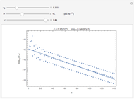
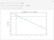
Snapshots

Details
This Demonstration shows how the distance between an orbit  of the logistic map starting at
  and a perturbed orbit
  starting at
  evolves. The initial perturbation
  is the starting error
  . The error changes on average with a rate (the error amplification factor), so that the error after iterations is roughly given by
  (see [1, Section 10.1] for more details). The Lyapunov exponent is . The plot is of
  versus for an orbit starting at with perturbation and parameter
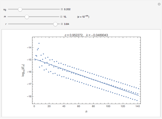
  . You can explore how changes with:
the starting value ,
the initial size of the perturbation ,
the parameter of the logistic map:  .
.
The Lyapunov exponent  is estimated by means of the slope of the linear fitting of . The expansion factor is
  , and . (This exponent is better estimated by
  for
for  ; see the Related Link "Lyapunov Exponents for the Logistic Map" and [1]).
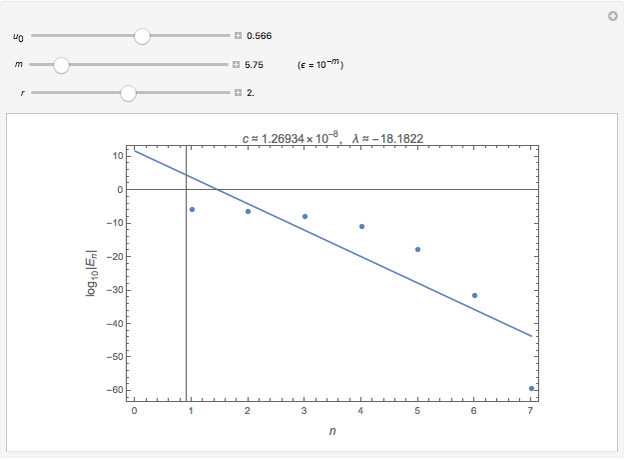
The iterations stop if  or
or  or
or  . The starting point of the perturbed orbit is
  if
if  .
.
Reference
[1] H.-O. Peitgen, H. Jürgens and D. Saupe, Chaos and Fractals: New Frontiers of Science, 2nd ed., New York: Springer, 2004.
Permanent Citation
 Feigenbaum's Scaling Law for the Logistic Map
Ki-Jung Moon Iterates, Cycles, and Bifurcations of the Logistic Map
Bernard Vuilleumier Variations of the Gingerbreadman Map
Erik Mahieu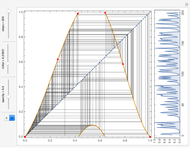 Time Series and Cobwebs for Arbitrary Recursive Maps on the Unit Interval
Vitaliy Kaurov Bifurcations of the Logistic Map
Rob Morris Controlling Chaos on the Logistic Map
Housam Binous Martin's Map Artwork
Erik Mahieu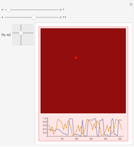 The Baker's Map
Enrique Zeleny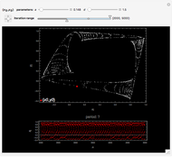 Iterations of Kaneko Map
Erik Mahieu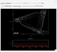 Iterations of Strick Map
Erik Mahieu
-
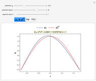 Eigenfunctions and Energies for Sloped-Bottom Square-Well Potential
Santos Bravo Yuste -
 Sensitivity to Initial Conditions for the Logistic Map
Santos Bravo Yuste -
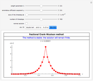 Numerical Solution of Some Fractional Diffusion Equations
Santos Bravo Yuste -
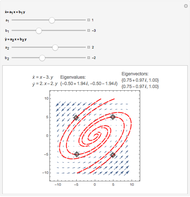 Phase Portrait and Field Directions of Two-Dimensional Linear Systems of ODEs
Santos Bravo Yuste