Tempered Fractionally Differenced White Noise


Requires a Wolfram Notebook System
Interact on desktop, mobile and cloud with the free Wolfram Player or other Wolfram Language products.
Tempered fractionally differenced (TFD) white noise  (
( ) can be defined using the backshift operator
  in the relation
  , where
  is Gaussian white noise,
  ,
,  and
and  is the series length. In this Demonstration, we consider the ranges of values:
  ,
,  ,
,  and
and  . This Demonstration explores the dependence on
  and
and  .
.
Contributed by: Ian McLeod, Mark Meerschaert and Farzad Sabzikar (September 2016)
(Western University, Michigan State University, Iowa State University)
Open content licensed under CC BY-NC-SA
Snapshots


Details
The selected range for the tempering parameter ,  , and the differencing parameter , , were chosen to exhibit a wide variety of time series behavior. When is large or is close to zero, they are almost independent. When is not too large and is not too small, there is a moderately strong dependence that can serve to model turbulent flow.
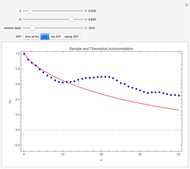
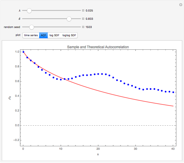
Snapshot 1: The sample and theoretical autocorrelations reveal the true structure and its estimate from the data. When the true dependence is strong, as in the case where is small and is not small, the sample estimates are not accurate and have large biases even in quite large samples. Due to this strong dependence, many spurious patterns in the sample autocorrelations may be generated. For example, setting "random seed" to 185 with  and
and  generates a spurious apparently periodic autocorrelation plot.
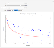
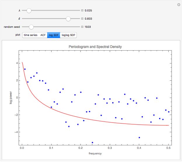
Snapshot 2: Log spectrum is plotted with the sample periodogram. The sample periodogram points scatter about the underlying theoretical value more randomly, illustrating that there is less bias than with the sample autocorrelation.
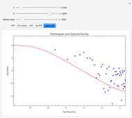
Snapshot 3: Log spectrum versus log frequency is plotted. The lowest frequency is chosen to illustrate that the TFD process has a bounded spectrum near the origin but obeys a power-law decay for intermediate frequencies.
The TFD model was suggested for turbulent flow in [1] and its extension to a more general family of models, denoted by  is discussed in [1] and [2]. This model is an extension to the FARIMA process.
References
[1] M. M. Meerschaert, F. Sabzikar, M. S. Phanikumar and A. Zeleke, "Tempered Fractional Time Series Model for Turbulence in Geophysical Flows," Journal of Statistical Mechanics: Theory and Experiment, 9, 2014 P09023. stacks.iop.org/1742-5468/2014/i=9/a=P09023.
[2] A. I. McLeod, M. M. Meerschaert and F. Sabzikar, "Tempered Fractional Time Series," working paper, 2016.
Permanent Citation
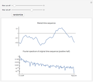 Filtering a White-Noise Sequence
David von Seggern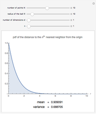 Distance Distributions in Finite Uniformly Random Point Processes
Sunil Srinivasa and Martin Haenggi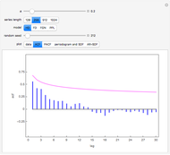 Time Series for Power-Law Decay
Justin Veenstra and Ian McLeod Aliasing in Time Series Analysis
Ian McLeod Informal Power Assessment of the Normal Probability Plot
Ian McLeod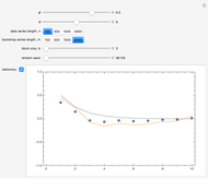 Block Bootstrap for Time Series
Ian McLeod and Leanna King p-Values Are Random Variables
Ian McLeod (University of Western Ontario)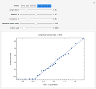 Monte Carlo Expectation-Maximization (EM) Algorithm
Ian McLeod and Nagham Muslim Mohammad Law of Large Numbers: Dice Rolling Example
Paul Savory (University of Nebraska-Lincoln) Goodness of Fit for Random Subsets
Michael Rogers (Oxford College of Emory University)