Autocorrelation and Partial Autocorrelation Functions of AR(1) Process


Requires a Wolfram Notebook System
Interact on desktop, mobile and cloud with the free Wolfram Player or other Wolfram Language products.
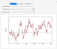
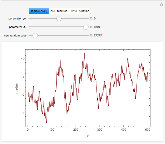
This Demonstration shows realizations of an autoregressive process of order one (AR(1)), its autocorrelation function (ACF), and its partial autocorrelation (PACF) function. The first tab, "sample AR(1)" shows realization of  :
:


Contributed by: Jozef Barunik (March 2011)
Open content licensed under CC BY-NC-SA
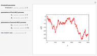
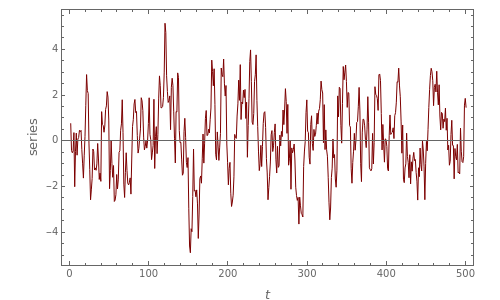
Snapshots


Details
An autoregressive process of order one can be described by:
 ,
,
where  is assumed to be white noise with
  . A simple autoregressive model of order one (an AR(1) model) has the same form as a simple linear regression model, where
  is dependent and
  is the explanatory variable, but they have different properties. The mean and variance conditionals on past returns are:
 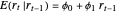 and
and 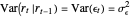 . Thus given the past return
  , the current return is centered around
  with variability
  . Assuming that the series are weakly stationary,
  ,
,  , and
, and  , where
  and
and  are constants. Necessary and sufficient conditions for the AR(1) model to be weakly stationary are
  ; otherwise the process is explosive. The ACF of
  satisfies
  for
for  , but as
  ,
,  , and the ACF of a weakly stationary AR(1) series decays exponentially with rate
  .
.
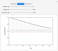
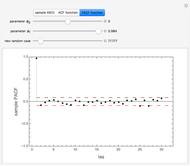
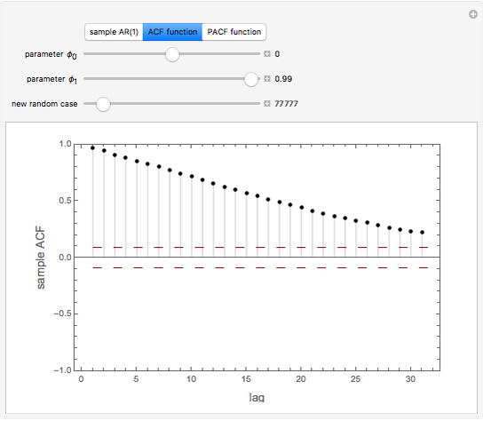
ACF and PACF are powerful tools for time series analysis. Snapshots 1, 2, and 3 show processes that are dependent (the parameter  is large); you can observe slowly decaying strongly significant ACFs, while the PACF shows only one lag strongly significant. On the other hand, snapshots 4, 5, and 6 show a negatively dependent process, where the ACF is decaying exponentially and the PACF has again only one significant lag. Note that the significant lag of the PACF points to the AR(1) dependence in the observed time series, while the sign of the PACF lag corresponds to the sign of
  .
.
References:
J. D. Hamilton, Time Series Analysis, Princeton: Princeton University Press, 1994.
R. S. Tsay, Analysis of Financial Time Series, New York: Wiley, 2002.
Permanent Citation
 Estimating a Centered Ornstein-Uhlenbeck Process under Measurement Errors
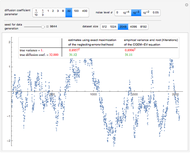
Didier A. Girard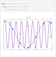 Aliasing in Time Series Analysis
Ian McLeod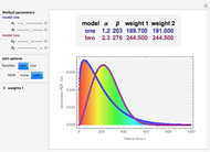 Comparing and Weighting Two Weibull Models
Frederick Wu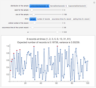 Records in Sequences of Random Variables
Heikki Ruskeepää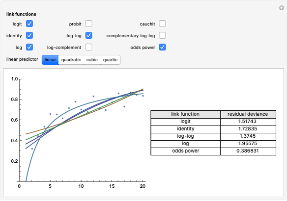 Comparing Binomial Generalized Linear Models
Darren Glosemeyer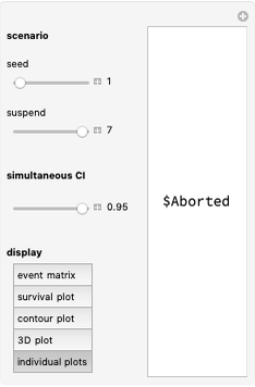 Simultaneous Confidence Interval for the Weibull Parameters
Michail Bozoudis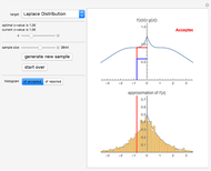 Acceptance/Rejection Sampling
Ryan Carroll and Jeff Hamrick 1, 2, 3-Parameter Logistic Rasch and Birnbaum Models and Item Analysis
Olexandr Eugene Prokopchenko Simulating the Poisson Process
Heikki Ruskeepää Simulating the Birth-Death Process
Heikki Ruskeepää