Acceptance/Rejection Sampling


Requires a Wolfram Notebook System
Interact on desktop, mobile and cloud with the free Wolfram Player or other Wolfram Language products.
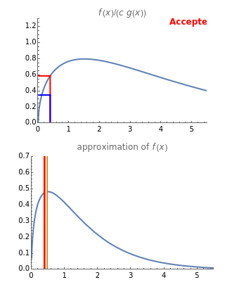
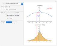
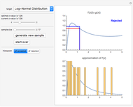
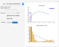
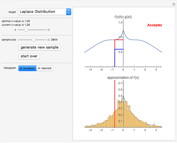
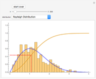
With this Demonstration, you can visualize the rejection sampling technique, which is also known as the acceptance-rejection algorithm. Select a target distribution (the distribution from which you would like to generate random samples) and then choose a "threshold value"  that influences the likelihood that a candidate sample from a nontarget distribution will be "accepted" as if it were, in fact, from the target distribution. You can change the number of random variates generated and view histograms of both the accepted and the rejected samples.
Contributed by: Ryan Carroll and Jeff Hamrick (September 2011)
Open content licensed under CC BY-NC-SA
Snapshots

Details
Suppose that you want to generate pseudorandom numbers from a random variable  with probability distribution
  , but that other methods (like the method of inverse transforms) do not work well (perhaps because the cumulative distribution function associated with does not have an explicit inverse). Instead, choose a companion random variable
  with probability density function
  , making sure that and have the same support (i.e. both vanish and fail to vanish over the same sets of real numbers).
Ideally, the random variable has been chosen in such a way that the cumulative distribution function associated with has an explicit inverse and is easy to simulate using a technique like the method of inverse transforms.
The acceptance-rejection algorithm is then as follows: (1) independently simulate a random number  with a uniform distribution over the unit interval and a realization * of the random variable ; and then (2) using a fixed, strictly positive number , accept * as a realization of if
  , where
  and
and  are the probability densities of the random variables and , respectively. If
  is not accepted, it is rejected. This process is continued repeatedly until a target number of realizations of is generated.
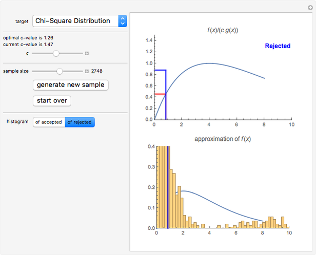
Heuristically, the acceptance-rejection method works particularly efficiently when certain conditions are satisfied. First, the target random variable and the companion random variable should have density functions that "look" as similar as possible. In this Demonstration, we use the exponential random variable as a companion random variable for the probability distributions with support on the positive part of the real line (the gamma distribution, chi-square distribution, half-normal distribution, and log-normal distribution). We use the Cauchy distribution as the companion distribution for the probability distributions with support over the whole real line (the normal distribution, the Student t distribution, the Gumbel distribution, and the Laplace distribution).
Second, the strictly positive constant influences the tendency of the algorithm to "accept" instead of "reject". If is particularly large, will be less than  with small probability, and the algorithm will throw away many fine proxies for . On the other hand, if is particularly close to zero and
  is not substantially smaller than
  , then will probably be accepted. It can be shown that the acceptance-rejection algorithm produces an empirical distribution of pseudorandom numbers that converges the most rapidly to the target distribution if is chosen to be the maximum possible value of
  over the (common) support of and .
The acceptance-rejection method can be generalized to the Metropolis–Hastings algorithm and is a type of Markov chain Monte Carlo simulation. For further information about the acceptance-rejection algorithm, see [1] or [2].
References
[1] S. M. Ross, Simulation, 4th ed., Boston: Elsevier, 2006.
[2] S. Ghahramani, Fundamentals of Probability, with Stochastic Processes, 3rd ed., New York: Prentice Hall, 2004.
Permanent Citation
 Sampling Theorem
Carsten Roppel Kernel Density Estimation
Jeff Hamrick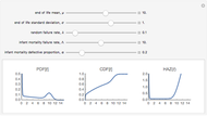 Closed-Form Full Life Cycle Distribution
Kelly S. Lowder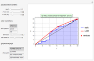 Estimating a Distribution Function Subject to a Stochastic Order Restriction
Michail Bozoudis and Vasileios Papachatzis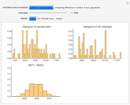 Bootstrap Percentile Confidence Intervals
Sijia Liang and Bruce Atwood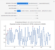 Records in Sequences of Random Variables
Heikki Ruskeepää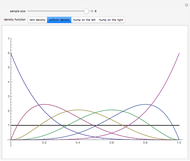 Distributions of Order Statistics
Chris Boucher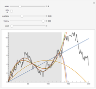 Polynomial Fits of Random Walks
Michael Schreiber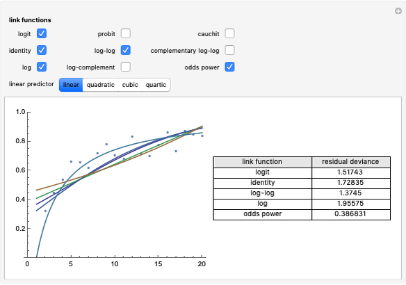 Comparing Binomial Generalized Linear Models
Darren Glosemeyer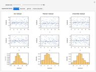 Comparing Some Residuals for Generalized Linear Models
Darren Glosemeyer
-
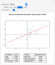 Expected Returns of the Dow Industrials, Beta Model
Jeff Hamrick -
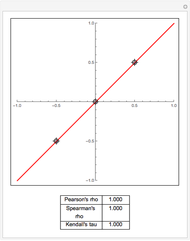 Exploring Measures of Association
Jeff Hamrick -
 Bootstrapping Credit Default Swap Data
Jeff Hamrick -
 Linear Dependence between Two Bernoulli Random Variables
Jeff Hamrick -
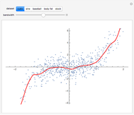 Estimating the Local Mean Function
Jeff Hamrick -
 Acceptance/Rejection Sampling
Jeff Hamrick -
 Simulating the 2008 U.S. Presidential Election
Jeff Hamrick -
 The Method of Inverse Transforms
Jeff Hamrick -
 The Perturbed Rat
Jeff Hamrick -
 Modeling Return Distributions
Jeff Hamrick -
 Pricing a European-Style Arithmetic Asian Option: Comparing Bootstrapping and Simulation Approaches
Jeff Hamrick -
 The Method of Common Random Numbers: An Example
Jeff Hamrick -
 The Envelope Theorem: Numerical Examples
Jeff Hamrick -
 Bootstrapping to Compute Value-at-Risk Standard Errors
Jeff Hamrick -
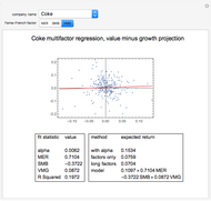 Expected Returns of the Dow Industrials, Fama-French Model
Jeff Hamrick -
Kernel Density Estimation
Jeff Hamrick -
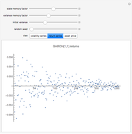 Simulating Asset Prices with a GARCH(1,1) Model
Jeff Hamrick